US congressional bill analysis, part II
This post is Part II of a two-part series based on LLM-assigned bill ambition scores for a subset of bills introduced in the United States Congress over the years 2011-2022. This post is designed to be fairly stand-alone, keeping references to Part I to a minimum.
Sections:
- Scoring overview
- Network analysis
- Predictive models for legislator scores
- Top scorers, House
- Top scorers, Senate
- Conclusions
Review of the data, in brief
The analysis of US congressional bills relies on a dataset of labeled and scored bills of certain significance over the 2011-2022 period. The bills are exclusively plain bills that at least made it into committee consideration. This amounts to about 10% of the total number of bills generated by Congress for that period. The downsample was chosen to avoid analyzing bills that had little serious chance of becoming law–these might include “moonshot” bills, or bills designed to act more as indicators on policy stances by the involved legislators.
Once the bills were selected, they were analyzed with the Anthropic Claude Haiku 4.5 LLM against prompt scripts, to return scope and depth scores, each in the range [0,10], as measures of bill ambition in the context of specific problems Americans deemed important. The problems, eight in total, were distilled from the Gallup polling company’s monthly “Most Important Problem” (MIP) surveys.
The per-bill scores were supplemented with additional data, including the legislative sponsor and any cosponsors. The per-bill data was also aggregated on a per-legislator basis, combined with legislator information like party affiliation and years of experience in the legislature. This resulted in two principal datasets:
- the per-bill dataset
- the per-legislator dataset
While Part I of this series primarily considered the per-bill dataset, Part II will consider the per-legislator dataset. This latter dataset allows forming, for example, per-legislator scores that gauge a given legislator’s performance on ambitious bills.
Summary of results for this post
Here’s a summary of main results of this post:
- per-legislator scores over a given calendar year were strongly tied to shifting party-dominance effects in the legislator’s chamber (House or Senate) when considering this set of ambition-oriented bills (scope*depth score > 9.0)
- unsurprisingly, party dominance effects corresponded to the majority party in the chamber of relevance
- the party dominance effect can be seen vividly in network plots, both static and animated
- year-to-year, and chamber-to-chamber, a given party can reach high levels of dominance, under some measures, which is strongly correlated to the number and ambition levels of bills produced by that party relative to the minority party
- if we define a “superstar” legislator as one who receives consistently high aggregated bill ambition scores over multiple year-chambers, then evidence for “superstar” legislators is minimal (though the possibility can’t be ruled out)
- global, per-legislator rankings, are provided at the end of the post–though there may not be any “superstar” standouts, we can nonetheless sort legislators based on finer gradations in their intra-year performances in the context of bill ambition levels
- a recurring theme of the analysis was inter-party balance; under this method of analysis and bill scoring, the US political parties were quite evenly matched over the 2011-2022 time period
Scores I
Scoring was accomplished in two phases
- per-bill scores, using the LLM-assigned scope and depth scores, relative to the bill’s associated MIP
- per-legislator scores, using an aggregate of per-bill scores for bills the legislator was involved in
We detail the phases below. Before that, a disclaimer.
Disclaimer:
Anyone can make a measure, but only some are useful.
General scoring schemes can be very subjective. In this case, in addition, is the subjectivity of the LLM in assigning ambition scores to bills, related, in part, to the ambiguities in LLM prompt instructions and wording. Reviewing the LLM-assigned scope and depth scores, at least the following two quirks were occasionally observed:
- the LLM assigned high scope and depth values, which are “correct” in the sense the bill is ambitious, but the outcome relative to the MIP (i.e. improving the problem Americans deem important) is ambiguous; for example, a bill that proposes addressing affordability concerns by enforcing broad price controls may provide short-term relief, but economists would probably agree the measure in the mid- and long-run would have the opposite effect
- the LLM assigned a high scope and/or depth score to a bill, but a human scorer would probably not set it quite that high; for example, a cybersecurity improvement measure scoring a scope and depth value of 4/10 on the MIP of jobs, but the jobs created by the bill would be limited narrowly to cybersecurity
While every effort was made to keep the scoring as meaningful and as simple as possible, the scoring method is in no way meant to be definitive, and most certainly would only apply in the context of the 8 Gallup poll MIPs (for instance, a legislator may have sponsored or cosponsored very useful bills in other contexts).
Per-bill scores
First, the scoring method assigned per-bill scores with the following formula,
bill score = mip_avg * scope * depth * prog_level/10.0,
with the factors,
- mip_avg–this is the average proportion of Gallup-surveyed Americans who listed the MIP as the most important problem facing Americans for that calendar year
- scope, depth–the LLM-assigned scores for the bill
- prog_level–bill progress codes were converted into numeric factors for scoring: ‘cmc’:0.5, ‘ooc’:0.6, ‘flc’:0.8, ‘flv’:0.9, ‘opc’:1.0
Per-legislator scores
To compute the per-legislator scores, in a given calendar year any bills that legislator sponsored or cosponsored were used for the scoring. The bill’s score was used without further modification if the legislator sponsored the bill. If the legislator cosponsored the bill, a cosponsor attenuation factor was used. The attenuation factor was specific to the chamber the bill was introduced in. The factor was determined from averaging the number of bill cosponsors per-bill in each chamber over the 12 year study period. The reciprocal of that factor was used. For the Senate, the factor was about 1/7, while for the House, which generally considers more bills, the factor was about 1/27. The resulting, weighted, bill scores were then simply summed for that legislator in that calendar year, to obtain the per-legislator score. The cosponsor down-weighting was used to normalize the effect of cosponsoring a bill relative to sponsoring a bill. In fact, it’s much more work to sponsor a bill in Congress than it is to cosponsor one, and without this normalization, there is a real risk a legislator who sponsored many ambitious bills would receive a lower general score than one who consponored many, but sponsored few.
Observe the distribution of the log of the per-legislator scores, by chamber. They look roughly normal, with perhaps some left skew.
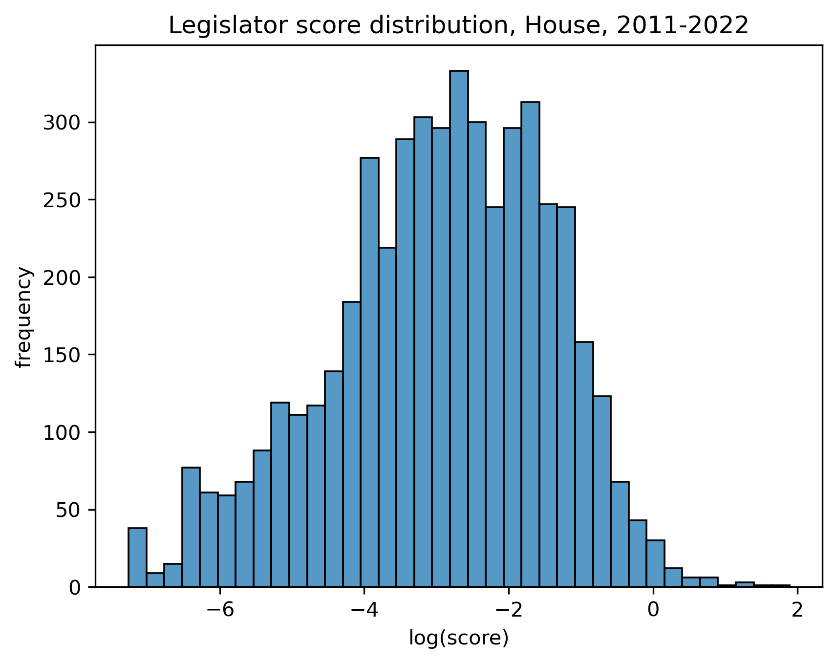
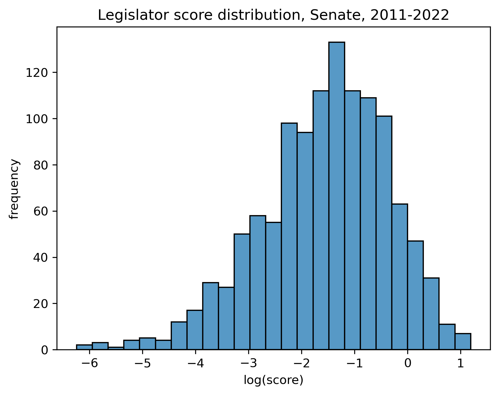
In association, by the properties of normal random variables, the histogram of the log of per-legislator scores for both chambers combined, also resembles a normal distribution (also with some left skew) (not shown).
In addition to general per-legislator scores, scoring was also calculated per MIP. For example, a legislator was scored only for their bills entailed in the MIP of healthcare. This allowed some measure of the ambition of bills associated with that legislator, narrowed to a specific MIP.
To analyze the per-legislator data, we’ll treat the chambers, House and Senate, separately. This is because, as just mentioned,
- the per-legislator scoring method used was dependent on the number of bills sponsored or cosponsored by any given legislator
- the House tends to introduce about 3 to 4 times as many bills as the Senate
So any comparison of scores between the House and Senate would then likely unfairly disadvantage the Senate.
Chamber dominance and networks
The per-legislator scoring scheme above, because it’s total summatory, is tied not just to the scores of the bills (and their MIP weights) a legislator is involved in, but to the number of bills as well. This was intentional, since a legislator involved with more bills at a given level of MIP ambition and significance than another legislator at those same per-bill ambition and significance levels, needs to sensibly score higher if the measure is to be useful. However, this creates a vulnerability in the scoring–legislator X could get involved with a few, very high quality bills, while legislator Y could get involved with a great number of low quality bills, and possibly exceed the overall score of legislator X. For this and other reasons, some exploration of intra-year-chamber dynamics will be helpful.
Chamber dominance
First, a look at bill participation levels by political party, within all the year-chamber combinations. We’ll look both at simple, per-legislator sponsorship counts, and at a more complex weighting that accounts for both sponsorship counts and (weighted) cosponsorship counts. These weights are summed by political party of the legislators, and depicted by year-chamber as bar charts. In agreement with the general scoring scheme, only bills with scope*amibition values greater than or equal to 9.0 were considered. We see a marked shifting of “dominances” in both chambers, with the effect much more pronounced in the House over our period of study (2011-2022) than the Senate.
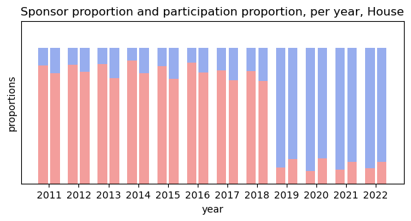
Proportion of sponsors (left bar, in a given year), and proportion of general bill involvement (right bar, in a given year) by party (Republican=red; Democrat=blue), House, 2011-2022
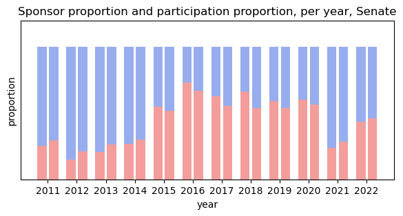
Proportion of sponsors (left bar, in a given year), and proportion of general bill involvement (right bar, in a given year) by party (Republican=red; Democrat=blue), Senate, 2011-2022
The bar charts and their shifting proportions make more sense when considering the chamber majorities.
House:
| years | majority party |
|---|---|
| 2011-2018 | Republican |
| 2019-2022 | Democrat |
Senate:
| years | majority party |
|---|---|
| 2011-2014 | Democrat |
| 2015-2020 | Republican |
| 2021-2022 | Democrat |
We’ll also check the average proportion over all 24 year-chambers in this 2011-2022 sample. By eye, the House is clearly dominated by the Republicans for 9 out of the 12 years. On the other hand, the Senate seems skewed toward the Democrats. In fact, the average Republican proportion, over all 24 year-chambers, for the sponsor proportions was 0.528, and for the general sponsor / cosponsor weightings was 0.509. Given the high inter-year-chamber standard deviation (around 0.30), this is clearly somewhat of a coincidence. But there are at least some reasons to support an eventual long-run inter-party balance in these proportions over more ambitious bills:
- election outcomes in the US, especially the past few decades, tend to be very close, leading to correspondingly balanced long-run chamber majorities, evidently a prime driver of the proportions
- Congress is fundamentally highly competitive, and, in association, parties compete with one another to capture maximal voting share
- the “voting market” is at least somewhat efficient (i.e. a voting republic with free-flowing information, and accurate representation of its citizenry)
Now, back to the concerns over the per-legislator scoring system. Some plots of the relative distribution of party bill participation as a function of bill ambition scores will serve as a coarse check on “cheating,” at least at a per-party level. For example, suppose in a given year-chamber, one party participates disproportionately over the other among lower-scoring bills, increasing their “score share” in a way that, perhaps, does not best serve the general constituency. We might also like to check if party dominance is associated with disproportionately more bills in the high ambition score range. So we’ll drill down into two party-dominant year-chambers, using the same per-party bill involvement weights of the bar charts just above, and check how the per-party weights are distributed among bill scores.
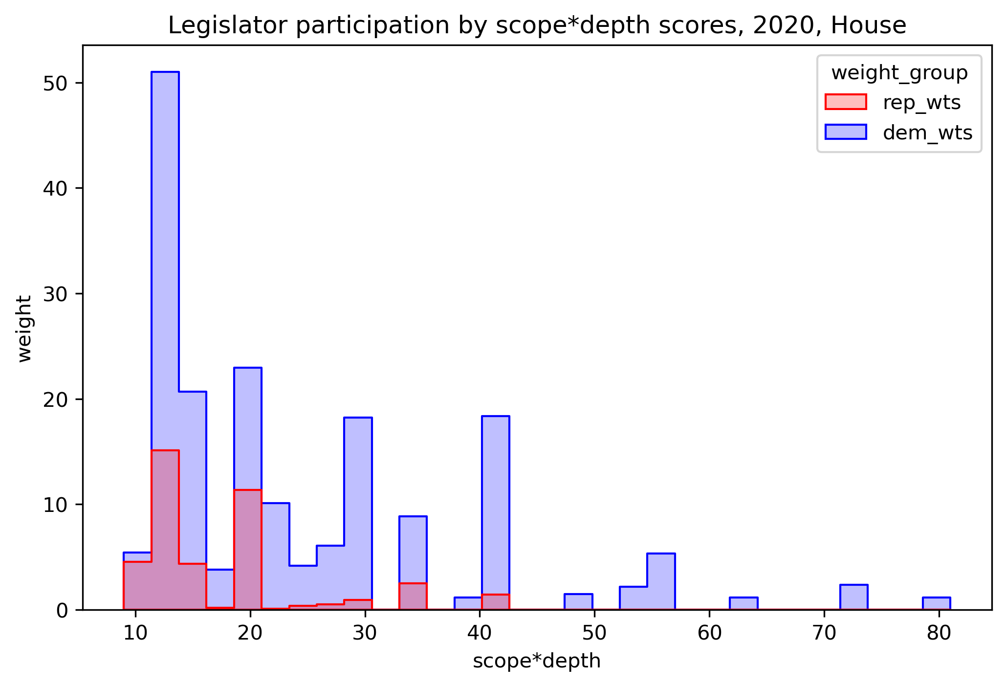
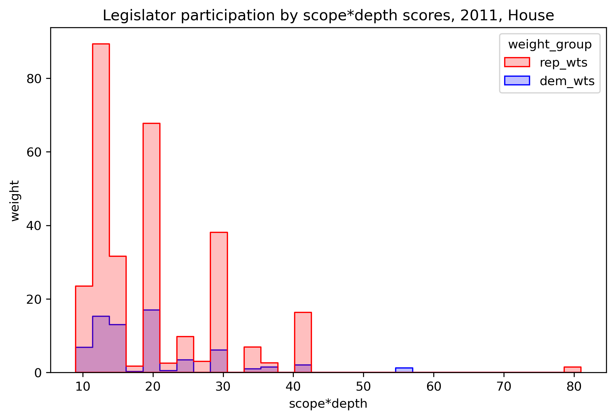
The dominance proportions appear to be fairly uniformly distributed over all bill ambition levels. A review of similar plots over all other year-chambers, and, overall, a similar uniformity persisted (not shown). This is somewhat reassuring for the sake of the scoring scheme.
Networks
The per-legislator scoring scheme and legislator bill participation above can also be viewed in the context of networks.
In this section, a few year-chamber networks are constructed by treating individual legislators as graph nodes and weighting each edge between legislator node pairs by the number of bills those two legislators were both involved in: “involved” meaning they each were either a sponsor a cosponsor on the bill.
The networks are then plotted by using the Fruchterman-Reingold “spring physics” algorithm: each legislator-node is given a natural repelling force, while a tension-spring-like attractive force is given between each pair of legislators in proportion to the weight of the edge between them (i.e. co-involvement sponsor / cosponsor count). This results, in general, in a legislator pair drawing closer together if they jointly participated on a relatively large number of bills, and remaining more separated if their co-involvement on bills is relatively low. It’s important to note that the Fruchterman-Reingold algorithm is not determinstic; it depends on a random seed, and the layout will differ run-to-run if the seed is not kept constant. So the network plots here are more for qualitative information than depictions of canonical, deterministic network structures in the year-chambers shown.
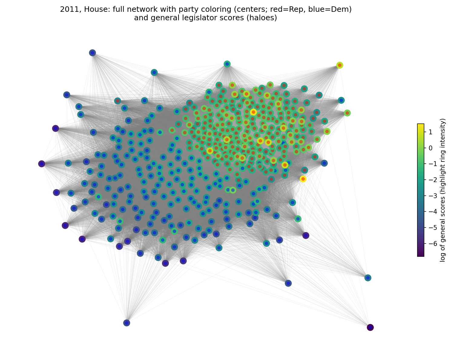
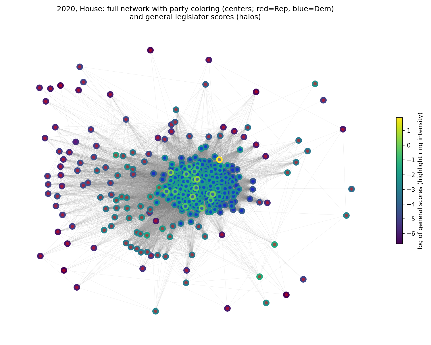
Sponsor / cosponsor network plots, 2011, House, and 2020, House; the plot on left shows tight clustering among nodes with red centers (Republicans), and the plot on right shows tight clustering among nodes with blue centers (Democrats); legislator scores (halos) in each are evidently higher among legislators in the respective clustering party
The initial pair of plots shows year-chambers that exhibited tight clustering, reflective of party dominance in the bar charts above, namely the bars corresponding to the House in years 2011 and 2020. Not every year-chamber shows such marked clustering. Consider the House in 2017.
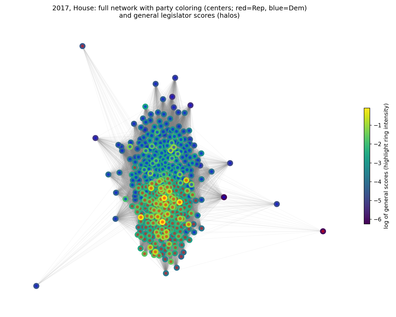
A sponsor / cosponsor network plot for the House, 2017; note that while the clustering seems more evenly balanced between Republicans (red centers) and Democrats (blue centers), the per-legislator scoring is noticeably higher among Republicans (halos)
The network plots shows a much less obvious clustering effect, yet the Republicans have a noticeable per-legislator scoring edge, by the spectral coloring of the node halos.
We’ll consider two more plots. Up to this point, we’ve only been inspecting the general year-chamber per-legislator scores, taken over all MIP topics. On the other hand, the two following plots correspond to MIP-specific scores. They were generated by simply aligning the per-legislator score node halo coloring scheme with the MIP-specific scores of interest. Note, the network structure was “frozen” from the co-involvement weights over all the bills (not just the bills associated with the given MIPs).
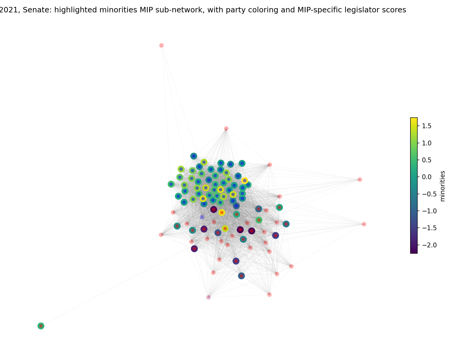
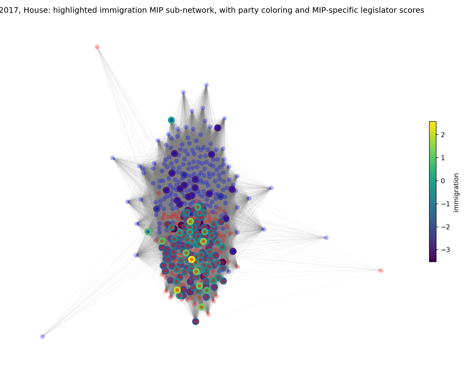
Sponsor / cosponsor network plots; on left, 2021, Senate under MIP minorities; on right, 2017, House, under MIP immigration; the plots show specialization under the MIP-specific scores
The plots serve to highlight party specialization effects. In both cases, a majority of nodes from the non-MIP-aligned party have no halos at all–this indicates those legislator nodes received no scores under that MIP for the year, having not participated in any bills at or above the scope*depth 9.0 threshold pertaining to the MIP in question. Specifically, we see the Democratic-specific attendance to the minorities MIP in the 2021 Senate, and the Republican-specific attendance to the immigration MIP in the 2017 House.
We’ll close the network section with an animation. This involves the running example of the 2011, House year-chamber. While the network plots above were static, aggregated over entire calendar years, what would the evolution of a network look like over the course of a congressional session? Would it show the same dominance effect as evidenced by the full-year plot? Or does party dominance fluctuate noticeably, changing hands over the course of a year, say, yet still strongly favoring one party on average?
To assess these questions, the entire 112th congressional session, effectively amounting to the yearas 2011-2012, was parsed at daily granularity. A corresponding series of network graphs was constructed on a 60 day sliding window. Each graph’s nodes were colored according to party orientation. Each window was successively fed to the spring physics algorithm as a slight adjustment to the previous window; this helped reduce large jumps between network renderings due to the vagaries of the non-deterministic algorithm. Some jumps, however, do remain–this is the result of, for example, big bills entering or leaving the 60 day window as the window slides forward, one day at a time. The bill density is sparse enough, that a single, big bill can cause a sudden realignment in the network nodes.
Another caveat to these windowed networks: this approach counts all the bill’s cosponsors on the day the bill was introduced. In reality, bill cosponsors tend to accumulate over the life of the bill. While I suppose it would be possible to fully augment the data with per-legislator cosponsor join dates, that was out of scope for this project.
Running the windows together in an animation, it looks, to me, a little like a time-lapsed cellular process. Note the periodic gatherings of dots around a circular perimeter–this corresponds to legislators with no sponsor or cosponsor links to other legislators via the bills in the animation frame’s time window.
We see that, for the most part, party dominance did not really shift intra-year–it rather remained with the party indicated by the upstream analysis (in this case, with the Republicans). This is consistent with a majority-party-associated driver of dominance, where the party retains its majority for the entire 2-year term.
Modeling and predictor attributions for per-legislator scores
Recall the per-bill score was derived from the straightforward linear formula from above,
bill score = mip_avg * scope * depth * prog_level/10.0,
while the per-legislator scores were created by summing relevant bill scores over all bills the legislator was involved in. So at the per-legislator level, the per-bill information has been “rolled up,” and the relationship between scores and predictors of interest gets more complex. This indirectness motivates this section, where we’ll examine the effects of several predictors of interest on the per-legislator scores.
One of the major questions, for scoring-usefulness purposes, has already been mentioned: how much does cosponsor involvement factor into the per-legislator scores? The network plots above, where edge weights were largely determined by co-cosponsorship levels betwen legislators, implied potentially high associations between cosponsorship and per-legislator scores. Given that the cost to a legislator of signing onto a bill as a cosponsor is quite low, the concern, again, is legislators can inflate their scores simply by cosponsoring more bills than their colleagues, and, in some sense, “cheat” under this scoring method.
Some of the other questions we’ll address in this section:
- What is the importance of Gallup-survey-derived yearly MIP importance, bill progress weighting, and bill ambition scores (relative) to other per-legislator bill score inputs?
- What is the relative importance (between each) of bill sponsorship and cosponsorship to the per-legislator scores?
- Is there evidence to support the idea of “superstar” legislators across year-chambers under this scoring dynamic?
To further motivate our exploration, we see the per-bill scoring formula heavily factored in both bill sponsorship and bill cosponsorship–with these moderated by the bill ambition scores, MIP weighting, and the bill progress level. Hypothetically, if the bill ambition scores, MIP weighting, and progress levels were purely randomly distributed, on average we’d expect the the party dominance displayed in the clustered bar charts above would tell the whole story.
To help address these questions, we’ll look at three models, in increasing order of complexity and decreasing order of interpretability:
- a basic linear model (OLS)
- a mixed effects model (linear)
- XGBoost
Then we’ll discuss and compare the results.
The basic, linear model
To establish a baseline, we’ll run a simple OLS model over all legislator scores, over all year-chambers. (Recall, the per-legislator scoring resolution is per year-chamber, per-legislator.) The predictors, chosen for relatively low inter-correlations, are,
- nsp_prp–a measure of chamber dominance (from the bar charts above): the party proportion, in [0,1], of bill sponsorships for that year-chamber
- num_spn–the per year-chamber, per-legislator bill sponsorship counts
- num_csp–the per year-chamber, per-legislator bill cosponsorship counts
The model:
log_score ~ nsp_prp + num_spn + num_csp
The results:
    Coefficients:
                  Estimate Std. Error t value Pr(>|t|)
    (Intercept) -3.9966222  0.0275184 -145.23   <2e-16 ***
    nsp_prp      0.9359763  0.0451253   20.74   <2e-16 ***
    num_spn      0.3981899  0.0093264   42.70   <2e-16 ***
    num_csp      0.0338436  0.0009272   36.50   <2e-16 ***
    ---
    Signif. codes:  0 ‘***’ 0.001 ‘**’ 0.01 ‘*’ 0.05 ‘.’ 0.1 ‘ ’ 1

    Residual standard error: 1.133 on 6084 degrees of freedom
    Multiple R-squared:  0.4896,	Adjusted R-squared:  0.4894
    F-statistic:  1946 on 3 and 6084 DF,  p-value: < 2.2e-16
| Df | Sum Sq | Mean Sq | F value | Pr(>F) | |
|---|---|---|---|---|---|
| <int> | <dbl> | <dbl> | <dbl> | <dbl> | |
| nsp_prp | 1 | 2608.398 | 2608.397731 | 2032.932 | 0.000000e+00 |
| num_spn | 1 | 3171.024 | 3171.024226 | 2471.432 | 0.000000e+00 |
| num_csp | 1 | 1709.486 | 1709.485767 | 1332.338 | 5.878459e-264 |
| Residuals | 6084 | 7806.208 | 1.283072 | NA | NA |
Even this basic linear model shows a fair amount of predictive power. The R2 is 0.49, with the ANOVA portioning for SS (given all its vagaries) showing bill sponsorship as the strongest component. That’s a good preliminary sign for the per-legislator scoring system, since we don’t want cosponsorship levels to dominate.
The mixed effects model
The basic linear model considers the year-chambers in aggregate. But because conditions on Congress may vary year-to-year in a way that entails some of our predictors, the predictor importance and significance may be inaccurately reported. For example, suppose some years presented demands on Congress that required a lot of bipartisan cooperation, while other years presented demands that favored clear party dominance. If considering party dominance (nsp_prp) as a predictor, the true effect of party dominance on the per-legislator score outcomes may be inaccurate.
A mixed effects model allows separating the effects of inter year-chamber variations on per-legislator score predictor relations. A mixed effects model, with its attributions of variance among random effects, also helps to address the “superstar” legislator hypothesis. If we model individual legislators as a random effect, then the model’s relative variance associated with that variable will provide information on how important individual legislator attributes are to the overall model fit.
Let’s first check the inter-year-chamber variations with some plots.
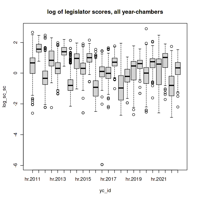
Distributions of the log of scaled and centered per-legislator scores, by year-chamber
The boxplots suggest a tendency for scores to cluster within year-chambers; but is this significantly different from what we’d expect of random samples from a normally distributed sub-population (as the log of the per-legislator scores appear to be)? Let’s look at one of the principal features, the year-chamber dominance scores, against the log of per-legislator scores, with color coding by year-chamber.
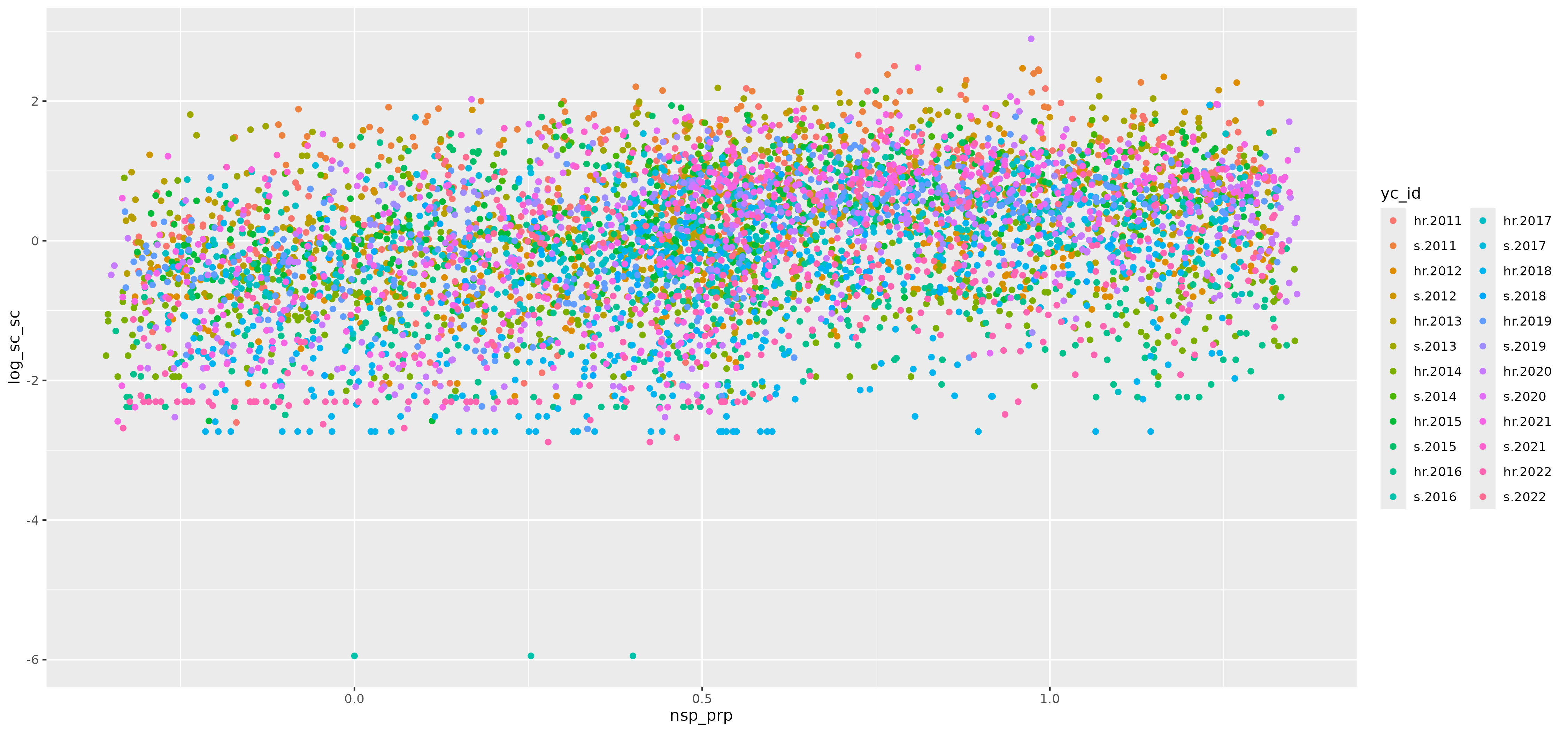
Any evidence of clustering within the region by year-chamber color coding suggests correlations within year-chambers between these main variables of interest. Clearly, something is going on, as certain colors show some non-unfirom clustering in different regions of the plot.
A mixed effects model can compensate for any intra-group correlations that may interfere with inter-variate relations of interest (here, the logs of number of sponsors and legislator scores), by assigning factors associated with those groups to random effects. The remaining variables are the fixed effects.
To run a mixed effects model, we’ll assign the year-chamber variable, and the per-legislator identifier variable (bioguide_id) to random effects. During model fitting, random effects are attributed to draws from a normal distribution–one distribution assigned to each random effects factor, where each level of each factor receives an intercept value to account for its (random) contribution to the output variable. The following diagram shows how the mixed effects models treats each of these 2 factors:
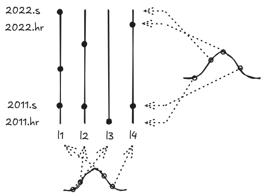
Shown are the two tiers of random effects in the mixed effects model: the per-year-chamber tier (vertical), and the per-legislator tier (horizontal); each tier's levels' intercepts are modeled as draws from a normal distribution
Note the two random effects impicitly require at least some legislators to be “crossers”–i.e. these are legislators who appear in more than one year-chamber. These are shown in the diagram as multiple node intersections, at various year-chambers, for each vertical legislator line (‘l1’, ‘l2’, …). In fact a vast majority of legislators satisfy this condition–for one, most legislators serve out their full two-year terms.
As a base model for mixed effects, we’ll start with a null model. This contains only the random effects–no fixed effects yet, other than a global intercept.
log_sc_sc ~ (1 | yc_id) + (1 | bioguide_id)
    Random effects:
     Groups      Name        Variance Std.Dev.
     bioguide_id (Intercept) 0.1308   0.3616
     yc_id       (Intercept) 0.4603   0.6784
     Residual                0.5210   0.7218
    Number of obs: 6088, groups:  bioguide_id, 965; yc_id, 24

    Fixed effects:
                Estimate Std. Error t value
    (Intercept)   0.2089     0.1399   1.493
We see the fitted model has assigned the two, expected normal distributions: one for year-chamber, with a variance of 0.46, and the other for individual legislators, with variance of 0.13. The residual variance in the random effects section tells us how much variance remains at the individual, unique, year-chamber-legislator level, after the year-chamber and legislator effects have been applied.
The relative variances in the random effects section tell us, proportionately, how much each element contributed. The between-level effects for the legislators was about 3.5 times less than the between-level effects for the year-chamber factor. The residual error was a little less than the sum of these two factors’ variances.
Fixed effects models don’t generally produce p-values, because they’re arguably not the right measurement for the model. So the variances, at this level of treament, are the main interest.
Next, we’ll fit a full model. To the null model, this adds fixed effects,
- the chamber dominance variable, nsp_prp, which recall amounts to per-year-chamber, per-party values
- the log of the year-chamber legislator bill sponsor counts (after adding 1, to prevent log() pathologies)
- the chamber designation (Senate or House)
log_sc_sc ~ nsp_prp + log1_ns + chamber + (1 | yc_id) + (1 | bioguide_id)
    Random effects:
     Groups      Name        Variance Std.Dev.
     bioguide_id (Intercept) 0.04156  0.2039
     yc_id       (Intercept) 0.23479  0.4846
     Residual                0.24793  0.4979
    Number of obs: 6088, groups:  bioguide_id, 965; yc_id, 24

    Fixed effects:
                Estimate Std. Error t value
    (Intercept) -0.97386    0.14074  -6.919
    nsp_prp      1.03900    0.02137  48.619
    log1_ns      0.73143    0.01392  52.562
    chambers     0.63347    0.19938   3.177

    Correlation of Fixed Effects:
             (Intr) nsp_pr lg1_ns
    nsp_prp  -0.078
    log1_ns   0.000 -0.283
    chambers -0.701  0.012 -0.029
Additionally, a plot of the residuals is provided.
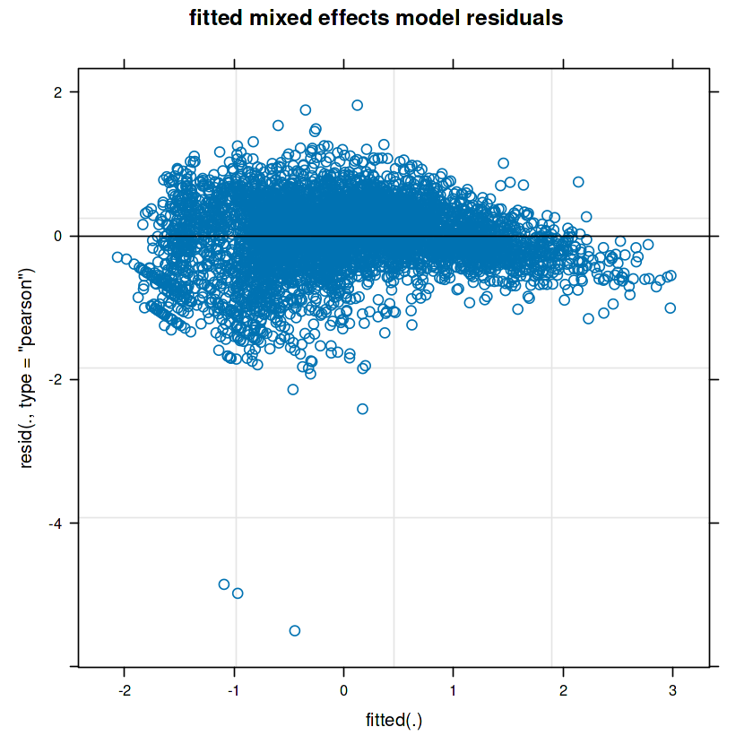
The residuals plot is admittedly imperfect, with a kind of comma shape. For what it’s worth, log scaling the number of times a legislator sponsored a bill helped improve it from an even worse shape. Since this is more or less an exploratory analysis, there will be no further attempts to address the evident hetereoskedasticity.
For the model variances, we’ll first compare the full model with the null model.
The random effects variance went from 0.6 in the null model (where there were no fixed effects) to 0.3 in the full model, which added fixed-effect predictors for the year-chamber party dominance measure nsp_prp, and the log of the number of bill sponsorships that year-chamber for the legislator, and the chamber factor (House or Senate). That indicates the fixed effects variables were appreciably predictive.
Additionally, the portion of variance attributed to the residual fell from 0.5 in the null model to 0.25 in the full model. This indicates the overall model, fixed effects and random effects combined, appreciably reduced the fit error.
For the full model on its own, note the decomposition of variance among the random effects. The variance attributable to between year-chambers was about 0.25, while the variance attributatble to between-legislators was about 0.05. The residual was about equal to their sum, at around 0.25. The relatively small proportion of variance attributed to inter-legislator differences suggests caution over ideas of “superstar” legislators. Of course, this model may not be the most appropriate for the situation. Relatedly, the residual, indicating what the model could not fit at the year-chamber-legislator observation level, was high relative to the between-legislator variance. That raises cautions in a signal-to-noise sense: the between-legislator variations may be, relatively, vastly different in a better-fitting model.
What might explain this preliminary lack of evidence for “superstar” legislators? It’s quite possible competitiveness comes into play: US Congress, as with any free political body, is fundamentally highly competitive, and true “superstars” may be constantly outcompeted. Additionally, there is the potential narrowness of the per-legislator score metric, and many competing inputs for legislators’ time and attention.
To close the mixed effects models section, while it might be natural to ask what the variance “explained” by the fixed effects of the full model is (relative to the random effects, or the total model fit), the literature is full of cautions on doing so, and we won’t do it here. (For example, a predictor can contribute to both fixed effects and random effects, making claims of fixed effects’ predictors contributing to some proportion of the overall model variance somewhat murky. For an entrypoint on further cautions see this link to a 2014 post on Cross Validated, which contains a rather long cautionary quote in context from Douglas Bates, the author of the R lme4 mixed effects library used above.)
What we can do is provide ordinary R2 for the full mixed effects model above, from a standard out-of-sample, cross-validated R2 metric. This has the additional advantage of allowing direct comparisons between models. The value is from R’s semEff package, and its R2() function,
R.squared.pred 0.73004506895676
Compare this to the very simple OLS above. The more complicated mixed effects model has improved the R2 roughly from 0.5 to 0.73.
XGBoost
The last model we’ll apply will be the most complex: XGBoost.
Since this model is adaptive to a wide range of predictor inter-relationships, we’ll provide both the per-legislator bill sponsorship and cosponsorship counts for the respective year-chambers. Additionally, both chamber dominance proportions will be supplied, the one addressing only bill sponsorships (nsp_prp), and the one combining sponsorship and (weighted) cosponsorship counts (nms_prp). To round out the predictor set, the numeric ‘year’ and factors ‘chamber’ and ‘party’ are also provided. We also predict on the raw per-legislator scores (not taking the log):
score ~ year + chamber + party + num_spn + num_csp + nsp_prp + nms_pr
The model showed an average cross-validation R2 of,
R2 ~ 0.85
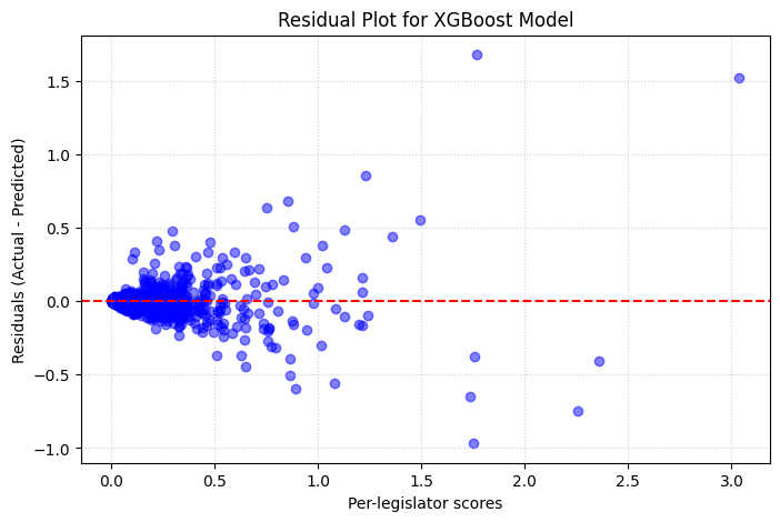
The residuals plot, additionally, showed much better accuracy for lower per-legislator scores than higher ones. This is somewhat expected, since the higher scoring legislators may be associated with a few sponsorships of very high scoring bills.
Feature importance was estimated via SHAP. The beeswarm plot indicated that sponsorship was the most important factor.
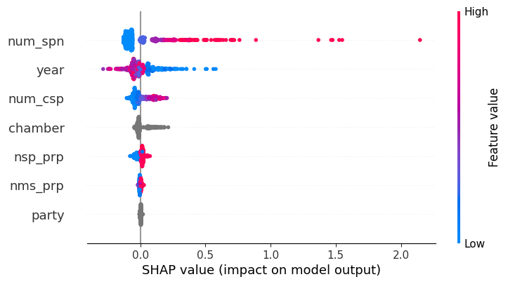
The associated feature importance weights from the model were: num_spn, 0.12; year, 0.06; num_csp, 0.05; chamber, 0.03; nsp_prp, 0.02; the remaining two, nms_prp and party, were effectively 0.0.
In agreement with the other models above, bill sponsorship counts dominate the predictors for impact on the legislator scores. Additionally, the relatively high R2 value, of 0.85, and the SHAP distribution indicate a lot of predictive power is being supplied by only a handful of predictors. Out of the 7 predictors applied, only 5 showed non-zero contributions by the SHAP algorithm. If, further, we give some credit to the mixed effects model, which “randomly” controlled for year-chamber, that leaves only the 3 numerics: num_spn, num_csp, and nsp_prp.
The accuracy is somewhat surprising given the absence of any information at the per-bill level–the level the per-legislator scoring was fundamentally based on. The model was supplied no information on the per-bill attributes that went directly into the per-bill scores: the yearly assigned MIP importance, the bill progress level, and especially the scope or depth scores.
Summary of per-legislator score models
From simplest to most complex, the three models showed improving predictive power, as measured by R2, approximately from 0.5 for the basic linear model, to 0.73 for the mixed effects model, to around 0.85 for the XGBoost model.
To address the questions posed at the beginning of this section:
What is the importance of Gallup-survey-derived yearly MIP importance, bill progress weighting, and bill ambition scores (relative) to other per-legislator bill score inputs?
The importance of those inputs, from the XGBoost model, appears to be subordinate to the per-legislator, per-year-chamber bill sponsorship counts, bill cosponsorship counts, and the party dominance measure. From the XGBoost fitted model residuals plot, which showed decreasing accuracy the higher the per-legislator score, those three bill score inputs–MIP importance, bill progress, and bill ambition–may be more significant the higher the legislator’s score. At the extreme, as mentioned above, sponsoring just a few highly ambitious bills may have a significant effect on a legislator’s overall score for that year-chamber: something none of the models above can capture since they do not have that information.
What is the relative importance (between each) of bill sponsorship and cosponsorship to the per-legislator scores?
Over all the models (implicitly for the mixed effects model: the model was more predictive when the sponsor count was used as a predictor, than when cosponsor count was used), the sponsor count variable had the greater influence. If going by the SHAP values for the XGBoost, roughly, the sponsor count variable influenced the per-legislator score outcomes by about twice as much as the cosponsor count variable. The primacy of the sponsorship variable over the cosponsorship variable helps address concerns of “cheating” by the legislators–i.e. of lazily signing on to a large number of bills as cosponsor, which may require very little effort, to increase one’s bill ambition score. Associatedly, we want the per-legislator scores tied strongly to sponsorship levels, since sponsorship requires the legislator do more “heavy lifting.”
Is there evidence to support the idea of “superstar” legislators across year-chambers under this scoring dynamic?
The primary model for insights into this question was the mixed effects model. Based on its results, there is not strong evidence to support “superstar” legislators across different year-chambers. This comes with the caveat that the linear mixed effects model may not be the best model for the question.
Scores II
Grand scores (scoring over multiple years)
In addition to per-year legislator scoring, scoring legislators over multiple years may be of interest. This, however, presents some challenges. From the per-bill scoring formula just above,
bill score = mip_avg * scope * depth * prog_level/10.0,
note that the mip_avg weighting could vary significantly year-to-year. In fact the total “mass” over all 8 MIPs of interest could also vary significantly year-to-year. While this is fine for intra-year score comparisons, this can create difficulties for meaningful inter-year scoring. Some methods to consider,
- normalize the mip_avg values between years: e.g. considering normalizing by the total “mass” for each year’s mip_avg values–but this would unfairly discount the importance of the MIP weightings for each year–for example, normalizing 2011 and 2012, where say MIP mass in 2012 was a fraction of what it was in 2011, would effectively diminish the importance of the MIP proportions within 2011
- just sum the yearly scores: this seems to make good sense since the per-year scores themselves were just sums (over whatever bills sponsored or cosponsored)–however, not all legislators served over the same set of years–so this creates overall comparison problems (e.g. suppose half of the legislators “missed out” on a “big” MIP year with lots of MIP mass–how to compare them to the legislators who did not miss out on the big MIP year?; in some sense, there’s no telling how any given legislator would have responded in a higher / lower MIP year than whatever they actually served)
- normalize the yearly scores themselves: scores could be normalized within each year, to make the distribution in some sense “consistent” between years; the challenge is in choosing a normalization method–as shown below, the distributions year-to-year for the per-legislator scores are not consistent (though they all somewhat resemble exponential distributions); some possibilities:
- normalize by the highest score each year–this suffers from the arbitrariness of high score outliers, as the score histograms just below indicate–the distributions have long tails with unevenly distributed outliers
- normalize by the total “score mass” each year, so that each year’s scores sum to 1–this can suffer from the apparent inconsistency in score distribution shapes year to year–for example, suppose two high-performing subgroups of legislators, one in 2011 and another 2012, have similarly high yearly scores among them, yet the scoring distribution is more highly weighted toward low scores in 2012 than 2011–then the legislators who happened to be in the 2012 subgroup see their high scores in some sense unfairly lowered
- rankings: another method is rankings–in other words first rank legislators within their chamber for a given year, then for inter-year scoring, just average the rankings; this has the advantage of simplicity, and avoids complexities in renormalization (and Congress is somewhat competitive, after all, so legislators may reference their performance off of that of others at any given time); a downside to this approach, however, is it ignores the relative magnitudes of per-legislators scores
As a compromise given all these considerations, we’ll use the rankings method, with the discussion serving as caution against investing too much in any single inter-year aggregation method.
House
We’ll start by applying the scoring schema to bills and legislators associated with the House.
Some plots of the distribution of per-legislator scores might be helpful. A few years are shown.
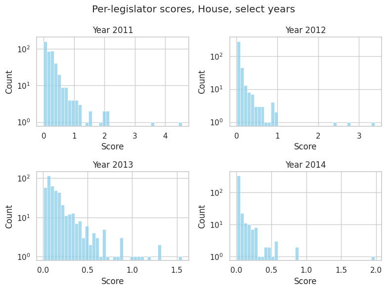
The plots show the scores are relatively unevenly distributed. Overall, they somewhat resemble exponential distributions (note the log scaling on the y axis).
To reduce variance in inter-year scores, and to ensure those scores are meaningfully linked to legislator performance, legislators who served for less than 4 years in the 2011-2022 timeframe will be excluded. To understand the effect, a plot of the distribution of years served will be helpful.
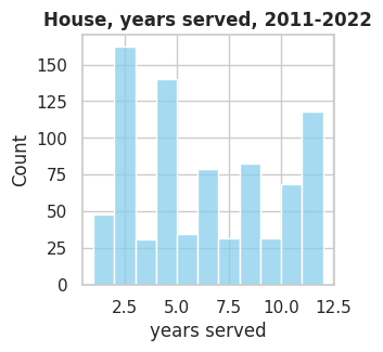
The cutoff will trim some 15-20% of legislators. We’ll accept that as a tradeoff.
The first step to developing scores will be assigning intra-year ranks. For each year, based on the House bill scores for each relevant legislator, we rank the legislators (from 1.0 being the best, 2.0 being 2nd best, and so on) based on their individual scores for that year. Next, we average the yearly rankings over years each legislator served. These rankings are then supplemented with more detailed per-legislator data, like age and years of experience, up to that point in time, as well as party afffiliation.
We can then see the top House legislators by this scoring system, along with some legislator details. Well just show the top 20:
| bioguide_id | avg_rnk | first_name | last_name | num_years | year_last | yrs_exp | rep_prp | age | |
|---|---|---|---|---|---|---|---|---|---|
| 61 | C000071 | 6.250000 | Dave | Camp | 4 | 2014 | 23.937521 | 1.0 | 61.482440 |
| 370 | M001197 | 8.500000 | Martha | McSally | 4 | 2018 | 3.986393 | 1.0 | 52.781371 |
| 115 | C001119 | 22.750000 | Angie | Craig | 4 | 2022 | 3.994606 | 0.0 | 50.881264 |
| 523 | S001216 | 27.500000 | Kim | Schrier | 4 | 2022 | 3.994606 | 0.0 | 54.358406 |
| 342 | M001144 | 32.333333 | Jeff | Miller | 6 | 2016 | 15.154315 | 1.0 | 57.517950 |
| 10 | B000013 | 39.250000 | Spencer | Bachus | 4 | 2014 | 21.936111 | 1.0 | 67.013012 |
| 197 | G000567 | 40.000000 | Tim | Griffin | 4 | 2014 | 3.989131 | 1.0 | 46.363717 |
| 327 | L000593 | 40.500000 | Mike | Levin | 4 | 2022 | 3.994606 | 0.0 | 44.178867 |
| 32 | B001273 | 43.500000 | Diane | Black | 8 | 2018 | 7.980999 | 1.0 | 67.960328 |
| 273 | K000363 | 44.166667 | John | Kline | 6 | 2016 | 13.957850 | 1.0 | 69.323805 |
| 387 | N000182 | 46.666667 | Randy | Neugebauer | 6 | 2016 | 13.549902 | 1.0 | 67.023964 |
| 398 | O000171 | 46.833333 | Tom | O’Halleran | 6 | 2022 | 5.993278 | 0.0 | 76.937925 |
| 484 | S000583 | 47.500000 | Lamar | Smith | 8 | 2018 | 31.921258 | 1.0 | 71.119872 |
| 107 | C001107 | 50.250000 | Carlos | Curbelo | 4 | 2018 | 3.986393 | 1.0 | 38.837211 |
| 177 | G000289 | 50.250000 | Bob | Goodlatte | 8 | 2018 | 25.927979 | 1.0 | 66.276515 |
| 259 | J000290 | 52.250000 | Lynn | Jenkins | 8 | 2018 | 9.971457 | 1.0 | 55.563085 |
| 580 | W000826 | 52.500000 | Susan | Wild | 4 | 2022 | 4.095909 | 0.0 | 65.570135 |
| 199 | G000569 | 53.000000 | Michael | Grimm | 4 | 2014 | 3.989131 | 1.0 | 44.898937 |
| 543 | T000483 | 53.250000 | David | Trone | 4 | 2022 | 3.994606 | 0.0 | 67.281327 |
| 47 | B001293 | 55.250000 | Mike | Bishop | 4 | 2018 | 3.986393 | 1.0 | 51.792987 |
The scores may some skew toward legislators who have fewer years served in the 2011-2022 time period. It might be easier to score more highly in the average rankings if having served fewer years–this from a naturally larger variation associated with averaging the rankings over fewer years. It could also indicate,
- legislators about to retire make more ambitious bills (i.e. they stopped serving sometime during the 2011-2022 window)
- relatively inexperienced legislators make more ambitious bills (they started serving during the 2011-2022 window, or served infrequently)
To check this, consider, for example, superimposed histograms, one for the top 50 rankings, and the other for the overall dataset:
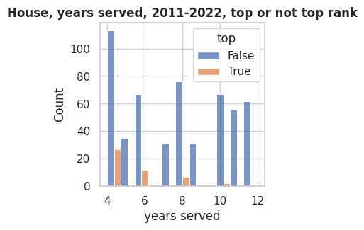
There does appear to be skew toward a lower number of years served in the top ranking legislators. How about for the lowest-ranked, bottom 50 legislators?
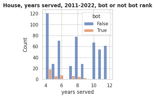
The lowest ranked also show some skew toward fewer years served, supporting the variational argument (i.e. fewer years served produces more variability in the average rankings). How do rankings relate to legislator overall years of experience?
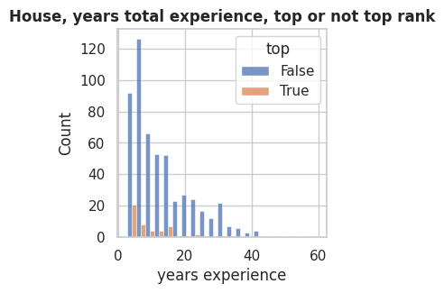
There may also be some skew toward lesser years of experience. Of course legislators with lesser years experience also likely served fewer years in the 2011-2022 timeframe. So this is somewhat ambiguous for the hypothesis that less experienced House legislators produce more ambitious bills, though there may be some evidence to suggest that. Let’s look numerically at years experience between the top 50 ranked, and the total dataset:
For House legislators with 4 or more years served in 2011-2022:
| overall average years experience | average years experience for top 50 |
|---|---|
| 13.048408477472728 | 9.29119694449578 |
The averages are notably different, and a t-test (Welch) indicates significance, p = 1.7e-4.
We can check Spearman’s r between the average rank and the years experience. The Spearman rank test gives significance (p = 4.76e-5) to the “paired” rankings–between the average rank of these legislators and the total years experience at the last recorded year they were active in the 2011-2022 period–but the r value is very weak: r = 0.17.
And for Spearman’s rank between average rank and years served in the 2011-2022 period, the r value is postive, but very week, r=0.10, with p=0.021.
Overall, it’s difficult to draw firm conclusions. The main questions, perhaps answerable with further study:
- how much of an effect does serving fewer years in the 2011-2022 have on average rankings, from variational effects alone?
- is there merit to the hypothesis that less experienced legislators tend to produce more ambitious bills in the House?
Senate
An identical scoring method will be used for the Senate.
First, as with the House, some plots of the distribution of per-legislator scores might be helpful. A few years are shown.
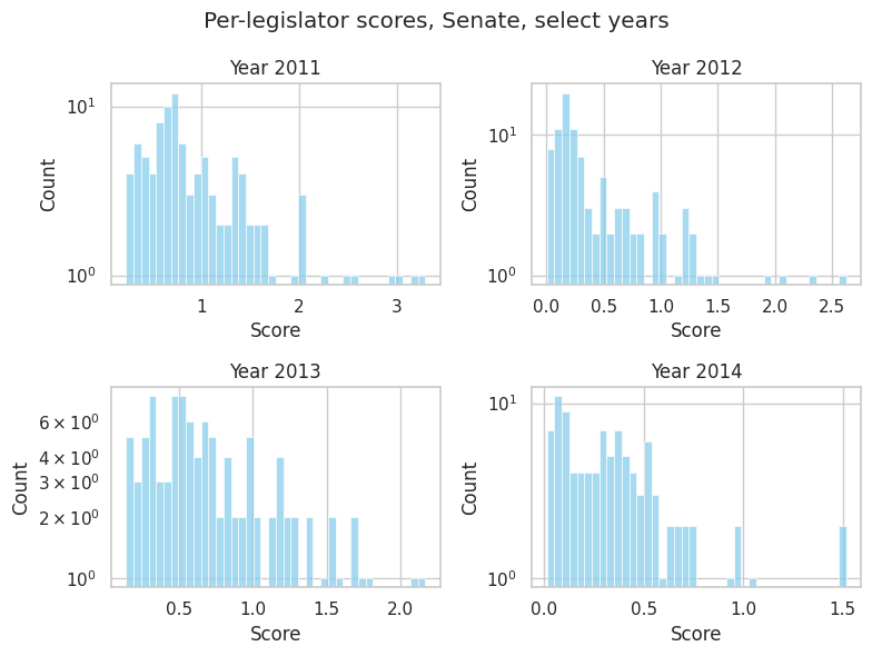
The Senate distributions of per-legislator scores are perhaps more regular than those for the House. It still appears difficult to fit these distributions “nicely” to an existing distribution, and there still appear to be high score outliers.
To reduce variance in inter-year scores, and to ensure those scores are meaningfully linked to legislator performance, legislators who served for less than 4 years in the 2011-2022 timeframe will be excluded. To understand the effect, a plot of the distribution of years served will be helpful.
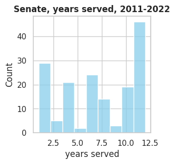
As with the House, this cutoff produces a loss of 15-20% of legislators, an acceptable tradeoff.
We duplicate the method of assigning and averaging intra-year ranks for each senator, according to their overall MIP bill ambition scores. Some detailed legislator data is then combined with the ranked lists.
We can then see the top Senate legislators by this scoring system, along with some legislator details. Again, we’ll just show the top 20:
| bioguide_id | avg_rnk | first_name | last_name | num_years | year_last | yrs_exp | rep_prp | age | |
|---|---|---|---|---|---|---|---|---|---|
| 48 | H000206 | 4.250000 | Thomas | Harkin | 4 | 2014 | 39.894043 | 0.0 | 75.119955 |
| 42 | F000457 | 16.428571 | Alan | Franken | 7 | 2017 | 8.479298 | 0.0 | 66.618753 |
| 72 | L000550 | 19.250000 | Mary | Landrieu | 4 | 2014 | 17.963408 | 0.0 | 59.108674 |
| 10 | B001265 | 20.250000 | Mark | Begich | 4 | 2014 | 5.985065 | 0.0 | 52.759468 |
| 55 | H001069 | 22.333333 | Heidi | Heitkamp | 6 | 2018 | 5.993278 | 0.0 | 63.174466 |
| 113 | S001203 | 24.666667 | Tina | Smith | 6 | 2022 | 4.991204 | 0.0 | 64.830900 |
| 117 | T000464 | 24.916667 | Jon | Tester | 12 | 2022 | 15.992115 | 0.0 | 66.364128 |
| 23 | C001035 | 26.250000 | Susan | Collins | 12 | 2022 | 25.955358 | 1.0 | 70.068516 |
| 66 | K000367 | 26.416667 | Amy | Klobuchar | 12 | 2022 | 15.992115 | 0.0 | 62.604982 |
| 12 | B001277 | 26.583333 | Richard | Blumenthal | 12 | 2022 | 11.989295 | 0.0 | 76.883167 |
| 82 | M001153 | 26.833333 | Lisa | Murkowski | 12 | 2022 | 19.975770 | 1.0 | 65.613941 |
| 107 | S001181 | 27.250000 | Jeanne | Shaheen | 12 | 2022 | 13.977015 | 0.0 | 75.927637 |
| 81 | M001111 | 27.666667 | Patty | Murray | 12 | 2022 | 29.971868 | 0.0 | 72.225987 |
| 49 | H000338 | 27.750000 | Orrin | Hatch | 8 | 2018 | 41.985804 | 1.0 | 84.782028 |
| 4 | B000944 | 28.500000 | Sherrod | Brown | 12 | 2022 | 29.949965 | 0.0 | 70.145178 |
| 25 | C001056 | 29.416667 | John | Cornyn | 12 | 2022 | 20.060645 | 1.0 | 70.914529 |
| 124 | W000779 | 29.500000 | Ron | Wyden | 12 | 2022 | 41.955687 | 0.0 | 73.666126 |
| 3 | B000711 | 33.000000 | Barbara | Boxer | 6 | 2016 | 33.966474 | 0.0 | 76.141194 |
| 9 | B001261 | 33.000000 | biologicalJohn | Barrasso | 12 | 2022 | 15.521195 | 1.0 | 70.449085 |
| 85 | M001176 | 33.500000 | Jeff | Merkley | 12 | 2022 | 13.977015 | 0.0 | 66.188902 |
In contrast with the House, here the years served in the 2011-2022 range actually skew toward the maximum value (of 12 years). A check of the Pearson correlation coefficient between the overall years of legislative experience and the per-legislator scores reveals a value of r=-0.104659.
Overall, the correlation is very mildly negative. Let’s check the average years experience in the top 20 against the total average:
| overall average years experience | average years experience, top 20 |
|---|---|
| 20.72883084526034 | 19.092274523143885 |
The average years experience is only slightly higher in the top 20 subset.
Conclusions
In this post, we saw the creation of a bill- and legislator scoring system, based on the MIP-specific LLM-assigned scope and depth scores for congressional bills. We then looked for correlations between those scores and predictor variables.
One major theme was the importance of chamber dominance, with party-majority dominance directly feeding into noticeably higher bill sponsorship and cosponsorship counts for the legislators of the dominant party, and with clear downstream effects on legislator bill ambition score splits over the parties in given year-chambers.
Network analysis emphasized the correlation between party dominance, mutual cosponsorship activity, and per-legislator scores. In some year-chambers, the subdominant party’s per-legislator scores were markedly lower en-masse, indicating a kind of overall atrophy in bill ambition for the party not in chamber majority. The network analysis also emphasized party specialization, to the point of exclusivity, for certain MIPs in certain year-chambers. In other words, for those year-chambers, members of one party or the other were almost exclusively responsible for ambitious bills focused on that MIP.
Modeling the per-legislator scores revealed a suprising amount of predictive power in just a few variables:
- a party chamber dominance measure, related to bill sponsorships
- the per-legislator bill sponsorship counts for that year-chamber
- the per-legislator bill cosponsorship counts for that year-chamber
The accuracy of that predictive power seemed to apply moreso to the lower-scoring legislators than the higher-scoring legislators. Presumably variables of greater interest in this project, those not included in any of the models, contributed important information to the higher scoring legislator’s scores. Those variables included ambition levels, bill progress, and MIP importance of the underlying bills the legislator was involved in–either as sponsor or cosponsor.
The mixed effects model provided some additional insight into inter-legislator and inter-year-chamber influence on legislator scores, when assigning those factors to random effects. The inter-year-chamber variance was an order of magnitude larger than inter-legislator variance. This refutes the idea of true “superstar” legislators, though the mixed effects model saw a relatively high proportion of variance in the residuals term, and better modeling of the fixed effects–non-linear models or variables not covered in the dataset, for example–might produce different and more meaningful variance splits.
A ranking-based global score for legislators in both chambers over the 2011-2022 period was generated, and the top 20 from each chamber were presented. For the House, after some preliminary analysis, we have a somewhat open hypothesis that less experienced legislators tend to produce more ambitious bills. For the Senate, the top 20 legislators skew toward those more experienced, as measured by time served in the legislator. Overall, however, the correlation between legislator experience and Senate rankings was very weak.
Party balance aspects
Part I indicated low to zero correlations between party affiliation and bill ambition scores. That neturality persisted at the per-legislator scoring level. Both the sponsorship and combined sponsorship/cosponsor mass party porportion bar charts showed fairly tight balance between the political parties. Also, the XGBoost SHAP scores notably do not assign much importance to party affiliation (here, coded as rep_prp variable) in determining per-legislator scores. In further addition, the top 20 global legislator rankings showed an almost even split between the two parties, with the House skewing toward the Republicans, and the Senate skewing by almost the same amount toward Democrats. This was clearly reflected in the party-majority dominance splits in those chambers over the 2011-2022 period.
As stated in Part I of this blog series, this balance is a desireable trait of the data gathering, pre-processing, and scoring system. In a highly competitive political environment, where polling consistently indicates the political parties are quite closely matched, any evidence of party-favoritism in the scoring system would be cause for concern.
Further questions and work
For the dataset overall, note that bill progress grading stops at the originating chamber–it does not track bill progress into the opposing chamber, which is a shortcoming of this work. For reference, only about 1/2 of bills that pass their originating chamber are passed by the complementary chamber, and only about 1/3 of bills that pass their first chamber are voted into law. Future iterations of the dataset could include opposite-chamber progress levels too.
Some per-legislator data was not included in the analysis, what may be of interest to some in its relevance on per-legislator scores. For example, does the state a legislator is from have any effect on their scores? and consider this, perhaps, in conjuction with other variables, like years experience?
Party majority dominance played a big role in year-chamber bill ambition output. This raises the question, what’s going on with the subdominant (non-majority) party and bill generation over various year-chambers? What characterizes, for example, the bills the subdominant party proposes? Are the ambition levels lower on a per-bill average basis, or are they about the same, with the main difference between the parties being the volume of output? Or does the subdominant party change tactics, and put its energies, say, into blocking bills the dominant party produces instead of focusing on bills of its own?
We might also consider a modified scoring system, which focuses on subdominant party bill output. Who, for example, are the “best” legislators given their party is not in majority, and what bills characterize their activity?
And, lastly, venturing, maybe a bit naively, into poltical science and legislative chamber health,
- is it “fair” the subdominant party is so evidently subordinated?
- is it wise to have roughly half your legislators so sidelined, with a marked dropoff, in some year-chambers at least, in their output of ambitious bills?
LLM usage disclosure
Outside of the obvious bill scoring, an LLM was used to help with this project at a few points:
- plots: I’m always happy to defer the finer details of plotting to an LLM (in this case, mostly the network plots)
- the dashboard: LLM chat sessions helped me understand the complexities of callbacks and fine-level control of elements in Plotly Dash
- the mixed effects model: this was a fairly new topic for me; chat sessions, combined with several respected (static) web pages on the subject, helped me understand mixed effects models and the interpretation of their results well enough to run and interpret mixed effects models used in that section