The lazy eater's problem

Or how to cut your food for maximal enjoyment

Introduction

Anyone who has eaten a crêpe, pancake, thin steak, calzone, quesadilla, etc., with a knife and fork may recognize the challenge: how best to cut off each bite? If you’re like me, you don’t want long thin strips, and you don’t want to pre-cut your food before eating it. So, how best to cut off bites to avoid those unappealing long thin strips?

Some formalism

Let the “lazy eater” be defined as someone, who,

• is eating a piece of food that we may regard as two-dimensional; for example, a pancake or crêpe might be idealized as a two-dimensional circle
• will consume the food in k bites of equal area, k an integer
• always cuts off the next bite in the following manner,
  • the cut must be made edge-to-edge on the remaining piece
  • the bite always consists exactly of what the eater just cut off
• considers their eating experience to be optimal if the bites they consume are as least oblong as possible

The last condition, on oblongness, again reflects a preference away from long, thin bites. For example, the eater would not eat a crepe or a thin steak by cutting off thin strips, but would prefer fairly round bites for the best eating experience.

There are many mathematical measures for oblongness, including, for example, the Reock score, and the Polsby-Popper score. For this project, the Polsby-Popper score was used. The Polsby-Popper score, or isoperimetric quotient, has been applied in measuring the sprawl of electoral districts, or voting areas, in the context of political gerrymandering. It’s a very simple measure of the compactness of a two-dimensional geometric shape. For a given two-dimensional shape with no holes in its interior, let A be the area of the shape and P the length of the perimenter. Then the Polsby-Popper score is calculated as follows:

\(\mbox{Polsby-Popper score} = 4 \pi A / P^2\)

Notice that if the shape is a perfect circle, the $A = 4 \pi r^2$, and $P = 2 \pi r$, producing a Polsby-Popper score of 1.0, which is the best possible score. The worst possible is bounded below at 0.0, where the perimeter approaches infinity with the area fixed. Figure 1 shows some other simple shapes and their Polsby-Popper scores.

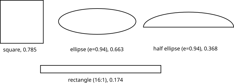
Figure 1: Polsby-Popper scores of some simple shapes

Notice the eater will not, for example, cut the food item in a grid pattern, then eat the resulting bites–even though that would be one way to help ensure the bites are as least oblong as possible. They will only make one edge-to-edge cut at a time, and will completely consume the fixed-area smaller piece (until down to the last two bites, when the cut-off piece will be the same area as the one remaining). Because they don’t make any “advanced” cuts in this sense, they are considered “lazy.” Most people would probably fall into this category.

In the mathematical abstraction, where the food item is considered a perfectly two-dimensional shape, we can ask questions like,

• for a given two-dimensional shape, to be cut into k bites in the manner specified, what is the optimal cut sequence to ensure all bites are as least oblong as possible?
• what shortcut strategies might be useful for the eater, to approximate an optimal eating experience without requiring complex calculations?

We can build algorithms to help answer these questions.

Existing work

Though a review of the literature did not reveal work directly similar to the lazy eater’s problem, there are a few major areas of tangency.

Stock cutting problem

Stock cutting (or cutting stock) problems refer to the general problem of (i) given a fixed-size sheet of stock, and (ii) a set of shapes to cut from the stock, what is the optimal arrangement of shapes on the stock, to minimize waste? - for example, a factory can only obtain cardboard stock in 4’ by 8’ sheets; they have a diverse set of shapes they need to cut from the stock, and want to minimize the waste, or trimmings, left behind after cutting out the shapes - this type of problem tends to be associated with operations research - the standard case may limit the cut-out shapes to rectangles

In general, stock cutting problems, at least in the case of rectangular shapes for cut-outs, are reducible to the knapsack problem, and are NP-complete. See for example [Avdzhieva].

Guillotine cutting sequences

A guillotine cut for a two-dimensional shape is a straight, edge-to-edge cut. A guillotine cut is not allowed to “stop” part-way into the two-dimensional piece, but must begin and end at the edges. When working with some materials, such as glass sheets, factory equipment may only allow guillotine cuts.

One may restrict a stock cutting problem to guillotine cuts. For example, the “2D sequential cutting stock problem” usually involves guillotine cuts (from the term “sequential”).

Relevance to this problem

In this case, the closest classification would be a two-dimensional cutting problem with irregular shapes, using guillotine cuts. See for example [Blazewicz], which treats irregular shapes, but using regular (not guillotine) cuts, or [Han], which treats fully-irregular shapes with guillitone cuts. However, of course, the lazy eater’s problem does not stipulate a set of pre-defined shapes to be cut out, but rather requires minimal oblongness for the cut-off bites.

Algorithms

The algorithms applied to this problem were simple, and arguably the “most obvious” algorithms to try. See the Discussion section for further thoughts on algorithm improvements.

Let $b_i$ be a bite, and let $P(b_i)$ denote the Polsby-Popper score of bite $b_i$. Recall $P(b_i) \in (0.0,1.0]$, and that a lower score means the piece is more oblong. Let $A_T$ be the target area for each bite. In all cases, the number of bites, $k$, was a positive integer, and if $A$ is the total area of the starting piece, then, obviously, $A_T = A/k$.

Two types of algorithms were used. Both involved “walks” around the perimeters of the two-dimensional shapes. A perimeter walk amounted to traversing the perimeter of the shape in equal-arc-length “steps.” Since, for all shapes, polygon approximations were used, computing such points on the shape’s (polygonal) perimeter was straightforward.

• greedy:
  • at each discrete point on the perimeter walk, make a guillotine cut, computing the cutting angle to get as close as possible to the target area for the bite being cut off, $b_i$
  • record the perimeter point, the cut angle, and the score $P(b_i)$
  • after a full walk around the perimeter, retain the point, cut angle, and bite associated with the maximal $P(b_i)$ (i.e. least oblong)
  • iterate until the area of the piece remaining is approximately the target area for the bites
• brute force:
  • for a given perimeter mesh, or step size, this considers every possible cut sequence
  • start with a uniform-step perimeter walk around the whole piece
  • at any point on the perimeter walk
    • make a guillotine cut, computing the cutting angle to get as close as possible to the target area for the bite being cut off, $b_i$
    • remove the bite
    • recurse with a new perimeter walk on the remaining piece
  • the nesting in the recursion ends when the area of the piece remaining is approximately the target area for the bites
  • apply an objective function to screen for and retain the “best” sequence from all the possibilities

For the brute force algorithm, the objective function needs to be specified. This requires some brief consideration, which we do next.

Objective function

For the brute force algorithm, we want to quantify what is meant by “as least oblong as possible” for the $k$ bites resulting from a sequence of $k-1$ guillotine cuts. Let $b_1,…,b_k$ represent the resulting bites. Two objective functions were utilized for the brute force algorithm:

• $O_a$: best average:
  • let cut sequence score $S$ be, $S = \sum_{i=1}^k P(b_i) / k$–i.e. take the average of the scores of the bites (*)
  • maximize S
• $O_w$: best worst:
  • consider the collection of scores, $C = {P(b_1),…,P(b_k)}$
  • order the scores in $C$ from lowest to highest, then to compare to the scores of another collection, $C’$, use lexicographic ordering; for example for ordered collections, $\{0.6,0.7,0.75\}$, $\{0.5,0.75,0.8\}$, and $\{0.6,0.72,0.74\}$, the ordering is, from worst to best, $\{0.5,0.75,0.8\}$, $\{0.6,0.7,0.75\}$, $\{0.6,0.72,0.74\}$ (noticing how, in the last 2, the least worst was tied at $0.6$, so the deciding scores were $0.70$ vs $0.72$, in the 2nd position)
  • retain the cutting sequence with the best score set under the lexicographic ordering

In general, after some experimentation, the best method appeared to be $O_a$. One problem with $O_w$ is it may over-weight the importance of avoiding a single highly oblong piece, while sacrificing potentially better scores for all the other pieces, especially when the number of bites, $k$, gets high.

(*) In practice, one further qualification was made to $O_a$. This was the result of rounding errors in computing the optimal guillotine cutting angle. For example, to save time there is some imprecision in the guillotine cuts used to produce a bite, resulting in slight inaccuracies between the area of the cut-off bite and the target area. At the end of the cutting sequence, this can result in a very small piece left over–for example, if the target area is 1.0, and each bite has area 0.99, then for 5 bites total, that leaves a small piece of area 0.05. Now consider objective function $O_a$. If every piece were weighted equally, regardless of size, then the last, small “extra” piece could have a very good value, i.e. a high value for $P(b_{k+1})$. But we do not really want that artificially raising the average. So an area penalty was applied in the average formula for $O_a$: each summand was further weighted by the area of the piece.

Cutting method

Since the algorithm can handle non-convex inputs, some details on how each guillotine cut is made are necessary.

For each perimeter point, the following cut method was used:

• apply a handedness rule
  • assume the perimeter walk proceeds in a clockwise direction around the shape
  • then the cutting angle will always be measured clockwise from the tangent ray at that perimeter point, with the ray pointing in the clockwise direction–this rule helps avoid double-redundancy in cuts (if the perimeter point was a vertex, then just use the tangent ray at a point slightly more clockwise–in fact only polygons were considered for input shapes, so this simply amounted to choosing the next polygonal segment, in a clockwise direction from the vertex, as the basis for the tangent ray)
• for non-convex “jumps,” choose the smaller bite
  • because non-convex shapes were allowed, it is possible for the area of the cut-off piece to jump, discontinuously, over a continuous change in cut angle; if the discontinuity contained the target area, then we can have a situation where the target area cannot be met with any precision (see Figure 2)
  • let a_l be the area of the cut-off piece just before the non-convex jump, and a_h be the area after the non-convex jump; if the target area is contained in the interval (a_l,a_h), then the algorithm always chooses the cut associated with the smaller area, a_l

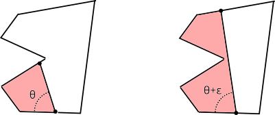
Figure 2: guillotine cut on a non-convex shape; a slight change to the cut angle can make a big difference in the area of the cut-off piece

Algorithms in code

These algorithms were coded in C++, with one program for the greedy algorithm, and one program for the brute force algorithm. The two programs shared a substantial amount of code. The main difference was that the brute force algorithm, for its perimeter walk routine, was made recursive, with one recursion level for each of the cuts.

Some notes on the implementations:

• While the brute force search is exhaustive, limited only by the step size used for the perimeter walk, it can also be quite slow. On a simple home Pentium CPU, without coding for a GPU and parallel processing, a 5- or 6-cut search with a starting step count of 30 for the outer perimeter, could take half an hour. Pushing beyond 6 or so bites for the finished piece became impractical.
• The greedy algorithm for the shapes studied here was generally quite competitive in $O_a$ scores at the measurable 6-bite range. Because the greedy algorithm did not require the time expense of recursive function calls, the step count for the outer perimeter walk on the initial shape could be set at 500 or more, and still finish at a fraction of the time of the brute force algorithm. Such a high step count, for the simple shapes studied here, ensured the scores for the greedy algorithm were near-optimal.
• When directly comparing greedy and brute force results on the same shape, the difference in step counts needs to be kept in mind. While the greedy algorithm operated nearly optimally, brute force, with its limit of around 30 to 40 outer steps for 6-bite pieces, could see more granular scoring. This granularity included the brute force score being 1% or 2% below the greedy score in some cases. Of course, the brute force score, at full precision, should never be below the greedy score, but computational constraints, translated into lower step counts, prevented obtaining such ideal results.

Let’s look at some of the results of these algorithms applied to some familiar shapes. (Note the figures here may not always render at the correct aspect ratio.)

Rectangles

First, let’s look at a square shape. Figure 3 shows the two algorithms side by side for comparison, using 5 cuts to make 6 bites total.

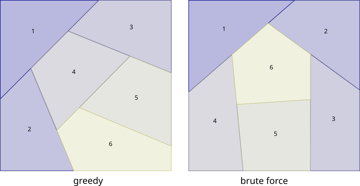
Figure 3: cutting a square into 6 bites of equal areas, greedy vs brute force; the cutting patterns differ slightly, and both $O_a$ scores were about 0.68

The two cutting sequences visibly differ slightly after the second cut. Both scores under the $O_a$ objective function averaging method, however, were nearly the same, at around 0.68.

Let’s retain the rectalinear configuration, and increase the aspect ratio. Figures 4 through 7 compare the greedy and brute force algorithms side by side, for width/height values of 1.2, 1.4, 1.6, and 1.8. (Noting, again, the figures may not render on the page true to their actual aspect ratios.)

Figure 4: cutting a rectangle, width/height=1.2, into 6 bites of equal areas, greedy vs brute force; $O_a$ bite-oblongness average scores shown

Figure 4 shows a width/height ratio of 1.2. The two cut sequences are very similar. The brute force score is slightly higher. Notice also a small leftover-piece artifact in the greedy segmentation. This, again, was due to rounding effects in the cut-determination routine, and should have a negligible effect on the overall score.

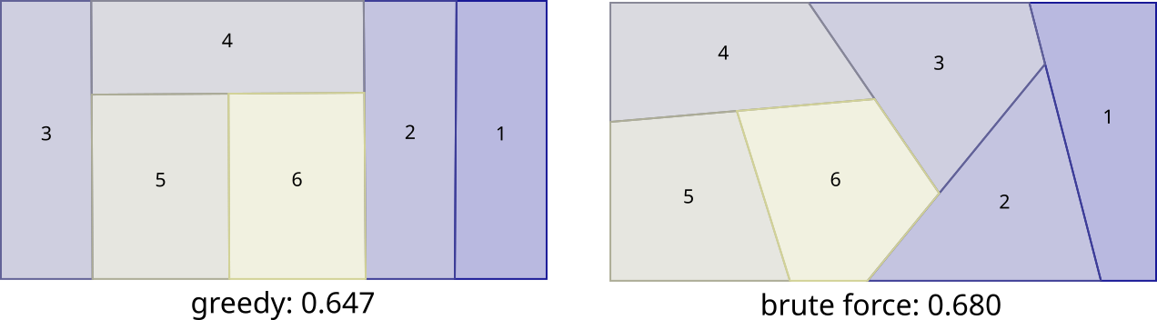
Figure 5: cutting a rectangle, width/height=1.4, into 6 bites of equal areas, greedy vs brute force; $O_a$ bite-oblongness average scores shown

Figure 5 shows the start of what looks a little like a phase transition. The optimal cuts seem to be transitioning from producing non-rectilinear bites, to rectilinear ones. This evidently is happening with the greedy algorithm first. With a little bit of thought, it’s easy to understand why such a transition should occur in some fashion:

• a square cut rectilinearly into 6 pieces would produce very oblong bites–surely we can do better, with triangular cuts for instance
• a rectangle with a high aspect ratio, on the other hand, seems most logically cut vertically into equal, lower-aspect-ratio rectangles–any other cut would only increase the oblongness score of the cut off pieces
• so somewhere between these extremes, gradually or suddenly, the cutting strategy should change over

An interesting side project might be to (a) determine if the transition is sudden, and (b) if so, figure the exact aspect ratio at which the transition occurs.

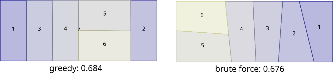
Figure 6: cutting a rectangle, width/height=1.6, into 6 bites of equal areas, greedy vs brute force; $O_a$ bite-oblongness average scores shown

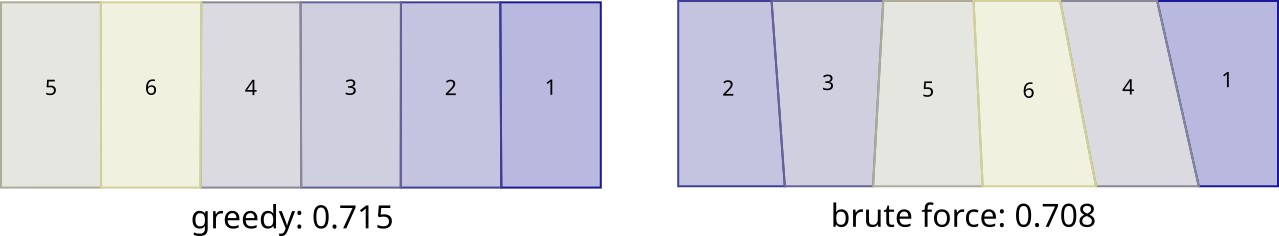
Figure 7: cutting a rectangle, width/height=1.8, into 6 bites of equal areas, greedy vs brute force; $O_a$ bite-oblongness average scores shown

Figures 6 and 7 show the brute force algorithm also settling down, until, evidently, at width/height=1.8, both algorithms seem to agree that making approximately vertical cuts at regular intervals is the best strategy for optimizing the bites. We note that though the brute force cuts are not completely vertical does not mean the optimal cuts are not–recall a relatively low step count was used for brute force at 6 bites, and if the step count were increased, the brute force cuts may become better vertically aligned.

Greedy unleashed

While the brute force algorithm is limited in the number of cuts it can make, the greedy algorithm is not so limited. This section will look at some shapes from the greedy algorithm under progressively higher bite counts. We emphasize that these cut sequences are not necessarily optimal, because the greedy method does not look ahead (at all).

The circle

Figures 8 and 9 show the results of the greedy algorithm on a circular shape.

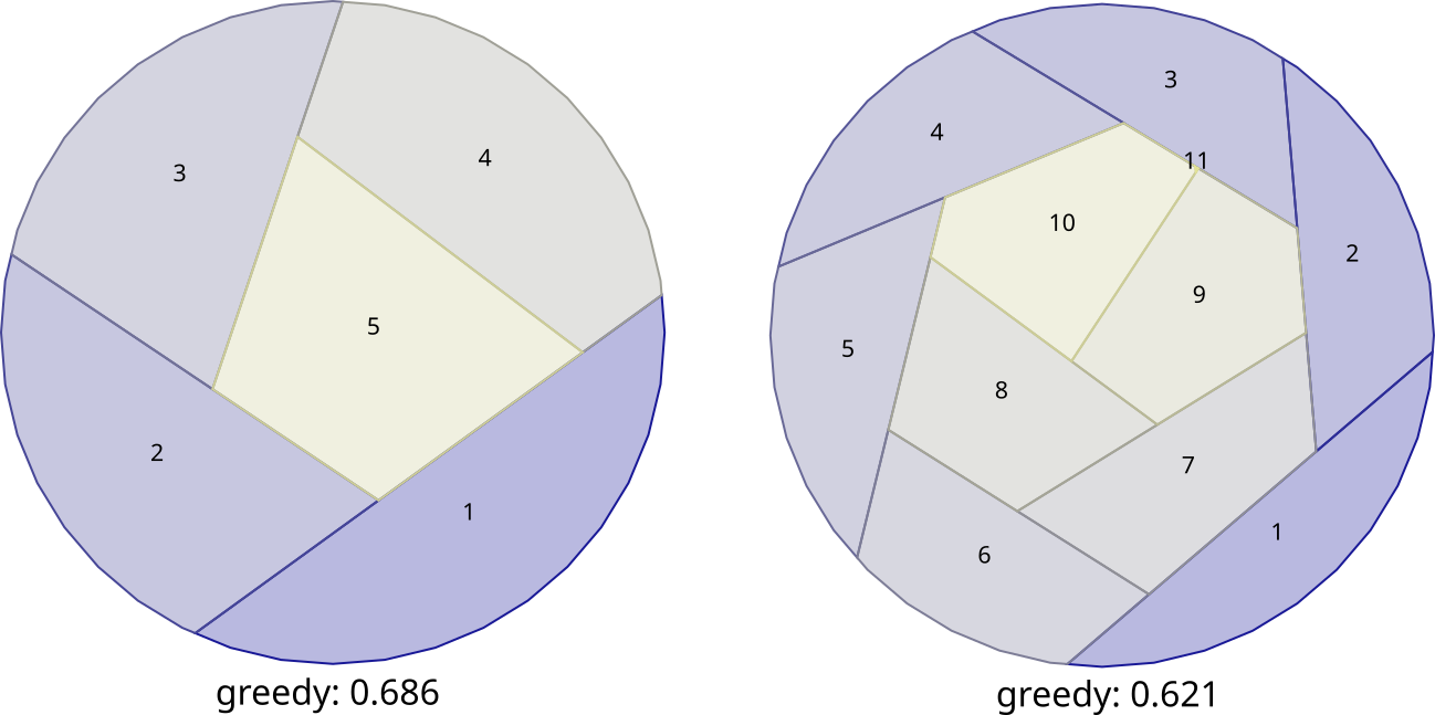
Figure 8: greedy algorithm with circles, at 5 and 10 bites; $O_a$ bite-oblongness average scores shown

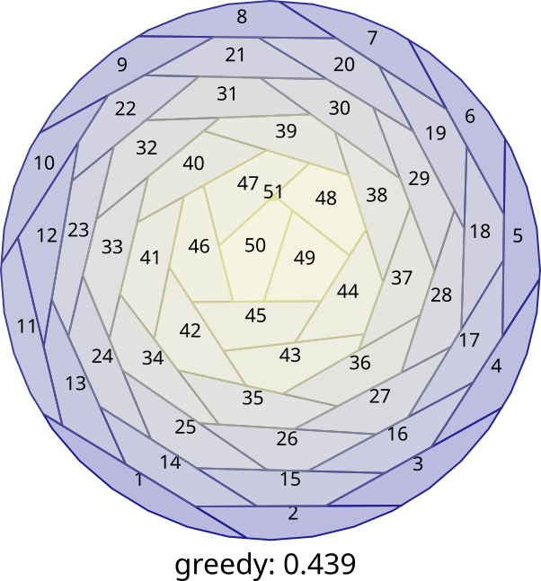
Figure 9: greedy algorithm, 50 bites with a circle; $O_a$ bite-oblongness average score shown

Two features of the greedy algorithm bite sequences for circles stand out:

• the average oblongness score drops as a function of the number of bites
• as the number of bites increases, the greedy algorithm tends toward a spiral cutting strategy (though with a few reversals in direction)

The tendency toward a spiral cutting strategy can be explained by two effects:

• because circular shapes have relatively constant local radii of curvature along their perimeters, the algorithm will exploit any advantage in slight variations in that curvature, relative to the size of the prospective bite
• the region adjacent to the most recent cut tends to have the most advantageous local curvature–i.e. such regions “stick out more,” on a scale comparable to the size of a bite

The ellipse

Figures 10 and 11 show the results of the greedy algorithm on an ellipse of fixed eccentricity.

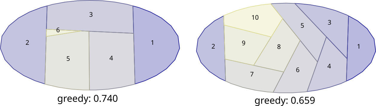
Figure 10: greedy algorithm with fixed-eccentricity ellipses, at 5 and 10 bites; $O_a$ bite-oblongness average scores shown

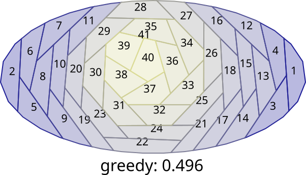
Figure 11: greedy algorithm, 40 bites with an ellipse; $O_a$ bite-oblongness average score shown

The cutting sequences for the ellipse tend toward a progression from the more sharply rounded left and right ends of the ellipse, toward the center. The progression is most pronounced for Figure 11, at 40 bites. In fact, the sequence starts in an oscillating pattern, alternately making a few cuts on one (left or right) end, then a few on the other. Once the process has produced a “circular enough” shape in the middle, a spiral cutting pattern dominates for the remainder, just as it did with the circles above.

The dumbbell

Figures 12 and 13 show the greedy algorithm applied to a dumbbell shape–i.e. two circles of equal radii connected by a rectangular bridge.

Figure 12: greedy algorithm with dumbbell shape, at 5 and 10 bites; $O_a$ bite-oblongness average scores shown

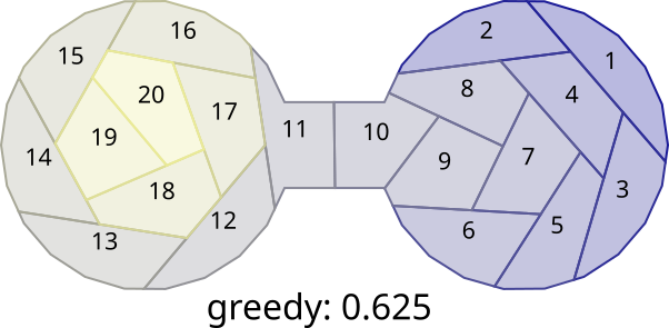
Figure 13: greedy algorithm, 20 bites with an dumbbell shape; $O_a$ bite-oblongness average score shown

At higher bite counts, the greedy cutting strategy favors processing one lobe of the dumbbell before the other. Additionally, the strategy differs between lobes. For the first lobe, the algorithm first removes bites that are not too close to the rectangular bridge. This can produce a cutting progression from the side of the lobe farthest from the dumbbell’s bridge, toward the bridge, and finishing at or with the bridge itself. This is at least somewhat intuitive, since the algorithm is prevented from going in a spiral around the first circular lobe because the bridge is in the way. So it has no choice but to remove pieces away from the bridge first.

Once the algorithm finishes with the first lobe, it processes the second lobe. Since the second lobe is now approximately circular, the spiral cutting pattern again emerges. This is especially evident in Figure 13.

Foiling the greedy algorithm

In the earlier examples of the rectangles with varying aspect ratios, it was clear that in most cases the greedy algorithm could be competitive with the much more computationally intensive brute force approach. It’s natural to ask: what are some shapes where the brute force algorithm is the clear winner over the greedy algorithm. Or, put another way, what kind of shapes can foil the greedy algorithm, and make it markedly inferior to optimal cutting strategies?

The shapes to help answer this question will be split into two categories:

• convex shapes
• non-convex shapes

Since it seems much easier to create non-convex shapes that will clearly foil the greedy algorithm, we’ll start with these first.

A non-convex shape to trick the greedy algorithm

In considering simple shapes, without convexity requirements and with a low number of bites, a good way to trick the greedy algorithm seemed to be to “protect” a region with very favorable (low oblongness) bites available by bordering the region with very unfavorable (high oblongness) bites. The greedy algorithm should avoid the unfavorable region, causing it to cut up the favorable region in an unfavorable way. Specifically, Figure 14 shows a favorable region of two squares being “protected” by two oblong rectangles–“two boxes on stilts.”

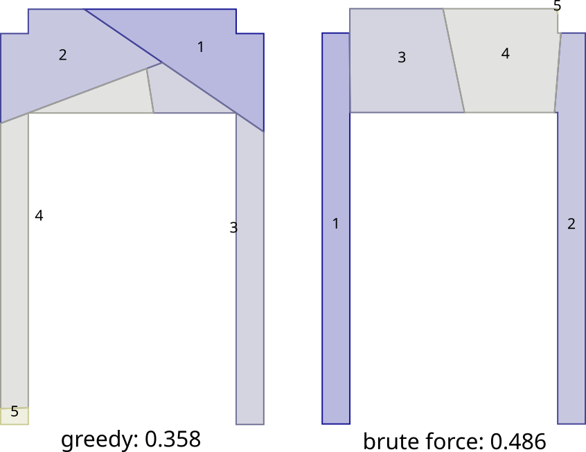
Figure 14: greedy vs. brute force algorithm, 4 bites with boxes on stilts; $O_a$ bite-oblongness average score shown

The shape was designed so that the optimal cutting sequence first removes each stilt, then cuts the adjoined squares into two separate squares. As Figure 14 shows, the greedy algorithm, in avoiding the oblong stilts at the start, cut up the two adjoined squares suboptimally. The brute force algorithm, to within its precision of an initial step count of 35 around the initial shape, found the optimum almost perfectly. In this case the greedy algorithm performed about 25% worse than the optimal cutting sequence.

I didn’t speed too much time devising non-convex shapes to trick the greedy algorithm. It’s probably relatively easy to come up with even more extreme examples of the greedy algorithm underperforming the optimal solution when non-convex shapes are allowed. Convex shapes, on the other had, seemed more difficult for this purpose and are the topic of the next section.

Convex shapes to trick the greedy algorithm

Because convex shapes don’t permit indentations, it was considerably more difficult to imagine convex shapes that can produce a large underperformance with the greedy algorithm. For example, the tactic of “protecting” a region highly amenable to low-oblongness cutting with very high oblongness regions, becomes challenging.

We’ve already seen some underperformance by the greedy algorithm, in the section on rectangles. Figure 5, at width/height ratio of 1.4, showed slightly less than 5% underperformance for the greedy algorithm relative to the brute force algorithm.

One shape that produced similar, but definitve underperformance in the greedy algorithm involved a house shape. The house shape started as a triangle (or “roof”) atop a rectangular base. The idea was similar to the boxes on stilts design, where a sharp, or “pointy” region (the “roof”) would cause the greedy algorithm to make sub-optimal cuts in other regions (the base of the house). Keeping the total figure area and the area of the rectangular base fixed, the apex of the roof was shifted in an arc around the base. This produced a series of house-like shapes with increasingly skewed roofs. The apex position that produced the largest underperformance by the greedy algorithm was retained.

Figure 15: greedy vs. brute force algorithm, 5 bites with skewed house shape; $O_a$ bite-oblongness average score shown

Figure 15 shows the result. The angle between the horizontal base line of the figure, and the line segment from the apex to the middle of the bottom of the base is about 70 degrees (again, the figures may not render on the page at their true aspect ratios). At around this angle, the optimum difference between the greedy algorithm and brute foce algorithm was achieved. In this case, the greedy algorithm performs a little more than 5% worse than the brute force’s presumed optimum. Notice how the brute force algorithm cuts off the pointy end (the top of the roof) first, while the greedy algorithm of course ignores this region as far into its sequence as possible. This produces a noticeable difference in bite shapes between the algorithms.

Discussion

Most of us probably instinctively use some form of the greedy algorithm when cutting “flat” types of food. Overall, the greedy algorithm appears competitive against optimal solutions when restricted to convex shapes. Non-convex shapes, on the other hand, can produce noticeably suboptimal results with the greedy algorithm.

Though not attempted by this author, given the foregoing, some useful variations on the algorithms might include:

• combine the brute force and greedy algorithms:
  • set a lookahead of k bites
  • for the given shape, run the brute force algorithm for only k bites
  • either remove all k bites as specified by the algorithm, or just remove the first j<k bites
  • recurse on the remaining piece
• greedy, brute force, or a hybrid, with protuberances first
  • this variant would look for protuberances, such as spikes, of area equal to or greater than the bite area
  • the protuberance would be handled first
    • if the protuberance was close to the bite area, it could simply be cut off
    • if the protuberance was more than about two bite areas, it could be cut with brute force, greedy, a hybrid, or even a lookup dictionary of shapes similar to the protuberance’s shape, where the cuts have already been computed
  • once the particular protuberance is handled, the process repeats
  • note, there exist software packages for identifying protuberances, such as opencv convexity defects in Python

In addition to improving the algorithms, the exposition above raised the following questions, which might be interesting to explore:

• how to explain the “phase transition” in the section on rectangles of increasing aspect ratios?
• what are some example of non-convex shapes that produce even greater underperformance by the greedy algorithm than for the two squares on stilts?
• under the restriction of convex shapes only, what are some of the absolute best convex shapes for foiling the greedy algorithm? can the underperformance demonstrated for the rectangle of aspect ratio 1.4, and the house with the skewed roof, be made worse?

AI usage disclosure: An LLM (ChatGPT) was used for preliminary research, to check if an idea of this type already existed in the literature, as well as for help with the C++ Boost.Geometry library.

If you found this post interesting, the source code is available here.

References

[Avdzhieva, 2015]: Avdzhieva, Ana & Balabanov, Todor & Kamburova, Detelina & Kostadinov, Hristo & Tsachev, Tsvetomir & Zhelezova, Stela & Zlateva, Nadia. (2015). Optimal Cutting Problem. (a technical report, fetched from https://miis.maths.ox.ac.uk/692/1/Optimal%20Cutting%20Problem.pdf, early 2026)

[Blazewicz, 1991]: Blazewicz, J. (https://pure.iiasa.ac.at/view/iiasa/1158.html), Drozdowski, M., Soniewicki, B., & Walkowiak, R. (1991). Two-Dimensional Cutting Problem. IIASA Collaborative Paper. IIASA, Laxenburg, Austria: CP-91-009. (fetched from https://pure.iiasa.ac.at/id/eprint/3571/1/CP-91-009.pdf, May 2026)

[Han, 2013]: Wei Han, Julia A. Bennell, Xiaozhou Zhao, Xiang Song; Construction heuristics for two-dimensional irregular shape bin packing with guillotine constraints; European Journal of Operational Research, Volume 230, Issue 3, 2013, Pages 495-504, ISSN 0377-2217, https://doi.org/10.1016/j.ejor.2013.04.048. (https://www.sciencedirect.com/science/article/pii/S0377221713003627)