Classifying raisins: Kecimen or Bensi?
The topic of this post is a classificaiton analysis for a machine vision raisins dataset. The dataset is the result of computer-assisted measurements of two types of Turkish raisins, Kecimen and Bensi. For each raisin, the researchers used a machine vision system to record 7 raisin parameters: area, perimeter, major axis length, minor axis length, eccentricity, convex area (the number of pixels enclosed in the convex hull of the raisin), and extent (“the ratio of the region formed by the raisin to the total pixels in the bounding box”). The dataset contains 900 raisin samples total and is perfectly balanced, with 450 of each type.
The goal of this analysis is to create a model to predict the value of the binary target variable, the raisin type. Because of the relative simplicity of the dataset, a correspondingly simple model was chosen for the analysis, with the use of decision trees. As it turned out, suitable feature selection was an important aspect of the problem: the dataset has a high proportion of redundant attributes.
An initial feature selection pass was made by selecting one feature at a time and training a decision tree just on that feature. For a measure of that feature’s predictive power, the difference in gini impurity scores was recorded. The gini impurity at the start was a uniform 0.5. This follows immediately from the dataset’s being perfectly balanced: a random draw would return a Bensi or Kecimen each with probability P=0.5:
\(\mbox{Gini before} = 1-P(\mbox{Besni})^2-P(\mbox{Kecimen})^2 = 1-0.25-0.25= 0.5\)
The resulting ordered gini impurites after training a tree on each lone attribute, under the restriction of a minimum leaf size of 20 (more on this later), were:
Perimeter: 0.18709817266105985
MajorAxisLength: 0.19295708458210944
ConvexArea: 0.2329118826603553
Area: 0.23745329204241425
MinorAxisLength: 0.3396154712016547
Eccentricity: 0.3425365538447386
Extent: 0.41913363859972214
Note the four attributes with the largest gini impurity reduction all have to do with the overall size of the raisin. In fact, it’s well-worth checking if these four attributes have correlations amongst them. Even though decision trees are capable of handling highly correlated attributes, all else being equal a simple model is favored over a more complex one. Paring attributes with redundant predictive power will help simplify the model.
Correlation analysis, both informally visually, and more formally with Pearson correlation coefficients indeed showed high correlations amongst all four of the attributes with the highest gini purity improvement. The correlation coefficients for select pairs were as follows:
\(\begin{eqnarray}
\mbox{ }&r&(\mbox{Area, ConvexArea}) = 0.99591967 \nonumber \\
\mbox{ }&r&(\mbox{Area, Perimeter}) = 0.96135172 (=0.94149339 \mbox{ if squaring the perimeter}) \nonumber \\
\mbox{ }&r&(\mbox{Area, MajorAxisLength}) = 0.93277443 (=0.91340292 \mbox{ if squaring the major axis length}) \nonumber \\
\end{eqnarray}\)
All four attributes are, unsurirpsingly, highly correlated. This combined with a little basic domain knowledge in geometry suggests there is little to be gained by selecting more than one of these attributes for training the decision tree model. So for training, we’ll select the attribute that produced the greatest gini impurity reduction of the four–this being the raisin’s perimeter.
Of the remaining attributes, minor axis length, eccentricity, and extent, all showed notably less predictive power when used as the lone attribute for the decision tree. Two of the attributes, minor axis length and eccentricity, have to do with the shape of the raisin. The fact they were less predictive suggests there is more intra-class variation for measures of raisin eccentricity than there is for measures of raisin size. As for the extent attribute, it was not clear if the bounding box around the image of the raisin was equally scaled for all the raisins. If it were equally scaled, then extent should have similar predictive power to area and the other three related attributes. Nonetheless, it was included as an option for final training.
To complete feature selection and tree complexity determination, fitting curves were plotted for various attribute combinations. The complexity of the tree was varied by varying the minimum leaf size, across the values 1,2,3,4,5,10,15,20,40,60,80,100,150,200,250,300. At each complexity level, 5-fold cross validation with random shuffling from sklearn’s model_selection’s KFold module was used and the accuracy averaged over all 5 splits. The best attribute sets in terms of test set accuracy involved one of the size-related attributes, with or without one of the eccentricity-related attributes. Indeed, the predictive power of perimeter alone was hard to beat. In the following figure, only the two attributes, perimeter and minor axis length were trained on.
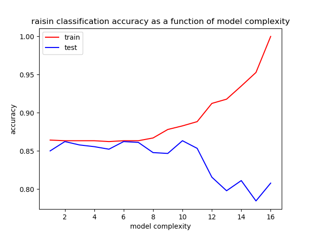
Figure 1: Fitting curve for the decision tree model using the attribute pair, perimeter and minor axis length. Complexity level corresponds to minimum leaf size in the {300,250,200,...} set of values.
Overall optimal accuracy is around the 7th to 8th complexity level, corresponding to a minimum leaf size of 40 to 60. (Recall the choice of the minimum leaf size of 20 in generating the single-attribute trees for attribute selection at the beginning; this complexity level seems a reasonable compromise between too complex and too little for attribute selection.) The accuracy at this level is a little more than 86%.
Note that with perimeter as the only attribute, the model at higher leaf size minima becomes extremely simple. The decision tree eventually amounts to a single interior node, which sets a decision value of around 1200 for the perimeter. The two resulting leaves correspond to Kecimen if perimeter <= 1200 and Besni if perimeter > 1200.
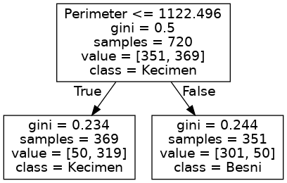
Figure 2: Decision tree using only the perimeter attribute, with a large minimum leaf size (300; low complexity).
If including an eccentricity measure, such as MinorAxisLength, the tree at higher complexity levels produced significantly more nodes, utilizing both perimeter and minor axis length as features. However, as the model complexity threshold is reduced, it eventually ignores minor axis length altogether, reducing again to just the perimeter.
Also note that because simple threshold works so well from the fitting graph(s), there’s very little apparent penalty on the test set for very simple decision tree models, as measured by minimum leaf size. This is not the usual behavior for a fitting graph. Normally, a very simple model would not fit the data so well, and the accuracy on the test set would improve as complexity was increased.
Overall, the classification exercise for this dataset, to within modest accuracy requirements, highlights the importance of attribute selection. After all the dust settled, we were left with a single, highly predictive attribute.
For the original study, see Classification of Raisin Grains Using Machine Vision and Artificial Intelligence Methods, Cinar et al1 (link, fetched December, 2022). In their analysis the authors used more sophisticated techniques–logistic regression, support vector machine (SVM), and a multilayer perceptron (MLP; a relatively simple neural network). They obtain an accuracy of 86+/-1% across all three of their models.
-
CINAR I., KOKLU M. and TASDEMIR S., (2020), Classification of Raisin Grains Using Machine Vision and Artificial Intelligence Methods. Gazi Journal of Engineering Sciences, vol. 6, no. 3, pp. 200-209, December, 2020. ↩