Automobile MPG predictions with linear regression
In this post, linear regression is used to predict automobile fuel efficiency, in miles per gallon (mpg), based on an archival automobile dataset from the 1970s and early 1980s, located here. The dataset consists of 398 entries. Each entry lists the name of a vehicle, along with eight other fields:
- number of engine cylinders
- total engine displacement (in cubic inches)
- horsepower
- vehicle weight (in pounds)
- acceleration (in English units, $ft/s^2$)
- model year
- origin (a discrete numbered field, roughly, American, European, or Asian)
- miles per gallon
(Note, the dataset had 6 rows with unknown values in the horsepower field; these rows were eliminated, leaving 392 remaining.)
First, the categorical variables in the dataset will be addressed. Categorical variables require special treatment in linear regression, since there is no guarantee different levels in the category in question correspond to linear differences in the dependent variable. The categorical variables in this dataset are, the number of cylinders, the model year, and the origin. To render a categorical variable suitable for linear regression analysis, it is converted into one or more indicator (aka “dummy”) variables. Each category of k levels will have a designated reference value and k-1 indicator variables.
To start with, we’ll address the origin field. This field corresponds to the region of manufacture of the vehicle. The category American will be the reference value, and we’ll have a European indicator variable (1 for European make, 0 for non-European), and an Asian indicator variable (1 for Asian make, 0 for non-Asian).
For the other two fields, cylinders and model year, a little more thought is required. The cylinders field could be left as a continuous variable, but caution is needed over whether the dependent variable (mpg) has a linear relation to the number of cylinders. The cylinders field could alternately be discretized, into, say, “low,” “medium,” and “high” groups with respective cylinder ranges (3,4), (4,5,6), (8). Then, this category could be split out into two indicator variables, with the most numerous (“medium”) the reference group. The question of which of these options to pursue will be postponed for now, addressed shortly when we consider multicolinearity in the dataset.
The last categorical field, model year, is even less likely to have a good linear relation to mpg. How might categorization help here? We’d like to split the year ranges into bins, and give the bins indicator variables, but how to choose the bins? Some research might be useful at this point. We can ask, what other inputs could affect a relation between model year and mpg? One obvious input would be national or international legislation. A little research in fact revealed some relevant legislation, the Energy Policy and Conservation Act of 1975, which mandated better fuel efficiency standards, starting with car models in 1978. So we’ll create a binary indicator, the model year category, using the split of model year $>=1978$, and model year $<1978$, based on this legislation.
Another consideration is the potential for multicolinearity in the input variables. Since linear regression will not work well if variables are too correlated, it is important to check for correlations between inputs. Even limited domain knowledge about automobiles would suggest several of the predictor variables are highly correlated. Horsepower, for instance, would likely be correlated with total engine displacement, which, in turn, would be likely correlated to the number of cylinders. A scatter matrix of the continuous variables can be used for a brief, informal, visual check of any stand-out correlations with the data.
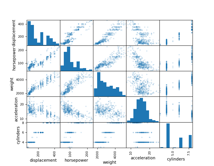
Figure 1: Scatterplot matrix of selected dataset attribute pairs.
This shows several of the expected correlations. A correlation matrix can give a more precise, quantative measure of the qualitative.
              displacement  horsepower    weight  acceleration  cylinders
displacement      1.000000    0.897257  0.932994     -0.543800   0.950823
horsepower        0.897257    1.000000  0.864538     -0.689196   0.842983
weight            0.932994    0.864538  1.000000     -0.416839   0.897527
acceleration     -0.543800   -0.689196 -0.416839      1.000000  -0.504683
cylinders         0.950823    0.842983  0.897527     -0.504683   1.000000
Clearly, one or more of the variables in this highly correlated group, horsepower, displacement, number of cylinders, and vehicle weight, should be eliminated. This may be further checked with variance inflation factor (VIF) scores. VIF scores have the advantage of pointing out not just pairwise correlations, but total correlations between a given test variable and the remaining variables in the regression.
                 VIF score
cylinders        10.630870
displacement     19.535061
horsepower        8.916017
weight           10.430271
acceleration      2.609487
All of these indicate high correlations between horsepower, displacement, number of cylinders, and vehicle weight. So we’ll retain only one of these four, vehicle weight, combine with acceleration and the two retained indicator categories, model year and origin, and check if that resolves the high VIF scores.
                   VIF score
weight             1.874747
acceleration       1.242865
model_year_ind     1.120857
European           1.362020
Asian              1.528470
That seems to solve the immediate multicolinearity concerns. This final paring also has the convenience of removing the cylinders field, eliminating any debate about making the cylinders field categorical or treating it as numeric.
It remains to train the linear regression model based on our pared attribute set of {weight, acceleration, model year (indicator), European (indicator), Asian (indicator)}.
Python’s statsmodel module was used. To avoid warnings of large condition numbers, the fields acceleration, weight, and dependent variable, mpg, were recentered about their means. The weight field was additionally scaled down by a factor of 1000, to keep its magnitude closer to that of the other variables.
                            OLS Regression Results
==============================================================================
Dep. Variable:                    mpg   R-squared:                       0.805
Model:                            OLS   Adj. R-squared:                  0.803
Method:                 Least Squares   F-statistic:                     319.5
Date:                Fri, 09 Dec 2022   Prob (F-statistic):          9.52e-135
Time:                        11:10:15   Log-Likelihood:                -1040.4
No. Observations:                 392   AIC:                             2093.
Df Residuals:                     386   BIC:                             2117.
Df Model:                           5
Covariance Type:            nonrobust
==================================================================================
                     coef    std err          t      P>|t|      [0.025      0.975]
----------------------------------------------------------------------------------
const             -2.7849      0.290     -9.611      0.000      -3.355      -2.215
weight            -5.8553      0.283    -20.726      0.000      -6.411      -5.300
acceleration       0.1654      0.071      2.336      0.020       0.026       0.305
model_year_ind     5.2421      0.381     13.750      0.000       4.493       5.992
European           1.7756      0.539      3.291      0.001       0.715       2.836
Asian              2.3369      0.539      4.332      0.000       1.276       3.397
==============================================================================
Omnibus:                       14.382   Durbin-Watson:                   1.149
Prob(Omnibus):                  0.001   Jarque-Bera (JB):               21.615
Skew:                           0.276   Prob(JB):                     2.02e-05
Kurtosis:                       4.009   Cond. No.                         11.0
==============================================================================

Notes:
[1] Standard Errors assume that the covariance matrix of the errors is correctly specified.
The R-squared value, reflecting the total fit of the model, was 0.805. All individual slopes were highly significant away from 0.
The model’s slopes show the variables with the largest effects. The weight category has a large effect on mpg. For every thousand pound increase in weight (recall our rescaling weight to thousands of pounds), the model predicts a decrease of 5.8 mpg. Another big effect is from the model year indicator variable. Taking a model year after 1978 improved the mpg by roughly 5. Since we already checked and fairly well-removed correlations with the other variables, it’s plausible the epochal mpg improvement had something to do with factors other than weight, acceleration, horsepower, displacement, or place of origin. It’s not unreasonable this improvement is the result of the legislation. Lastly, the vehicle’s place of origin had a statistically significant effect on mpg. An Asian make, improved mpg by 2.3 units over American cars, and a European make improved mpg by 1.8 over American cars. What the model does not directly indicate is how well Asian makes do relative to European makes. A little simple math produces,
\((\mbox{Asian-American}) - (\mbox{European-American}) = \mbox{Asian - European} = 0.56.\)
So Asian cars have a 0.56 mpg improvement over European cars under the model. Is this statistically significant? To test for significance, we can do a simple t-test, looking for significance between the average mpg’s of the European and Asian indicator variables. We get a p-value of 0.338. So we can’t really reject the null hypothesis that European and Asian cars have the same mpg.
This completes the analysis. As a final note, the large omnibus score of the model suggests the residuals are not normally distributed. A plot of the residuals, $y^{\prime}_i - y_i$, over all instances shows a relatively Gaussian-looking distribution. It’s possible the large omnibus score reflects the presence of outliers. A larger sample size might help, but there are obvious limitations since the total number of mass-produced vehicle models is itself limited. A little more research revealed the total number of distinct models in the US is typically in the hundreds, so we expect this sampling from the 70s-80s of around 400 global models to be fairly complete. Further analysis might reveal the actual reasons behind the large omnibus, which we do not pursue here.