Triangular billiards: plotting bounce sequences

Introduction

Mathematical billiards is the study of mathematical models of the familiar game of pocket billiards. At its most basic, the billiard may involve a point particle in inertial motion over a two-dimensional, pocketless, frictionless table, where the boundary collisions are perfectly elastic. A common simple table shape is a convex polygon. Classifying the orbit structures becomes even easier if the polygon has rational angles: that is, every angle can be expressed as $a\pi/b$ where $a,b \in \mathcal{N}$.

Often, the orbit phase space is studied. All of the dynamics can be accounted for with a first return, Poincaré map, which is only concerned with the billiard ball the instant it rebounds from a wall of the billiard table. The map only records the ball’s point of impact, via the oriented arc length from some reference point on the table boundary, and the velocity vector as it heads away from the wall toward its next collision. The entire billiard dynamics may be obtained from initial conditions under iterations of the map.

For rational convex polygons, abundant work has been done on the general well-dispersion of the orbits, including periodic orbits. In the case of rational polygons associated with Veech lattices, the general dynamics are particularly easy to categorize. For an in-depth treatment of rational mathematical billiards, see for example Masur and Tabachnikov [1].

Another approach to studying billiard orbits is to record the bounce sequence. The sides of the triangle are labeled, and the side struck at each collision is recorded. A bounce sequence is obviously less rich than the return map, but in fact it has been proved the billiard table can be reconstructed up to certain isomorphisms from its corresponding set of bi-infinite bounce sequences over the whole phase space [2],[3], or in the case of rational polygons from a single orbit under certain mild conditions [4],[5],[6].

For this post, billiards on rational triangles under a fixed number of collisions are considered. For an initial trajectory along a billiard wall, let $\theta$ be the positive angle between the trajectory and the wall under some fixed orientation, and $x$ be the foot point of the initial velocity vector along the wall. A phase space is formed by selecting the triangle’s longest side, of length $w$, and considering initial $(\theta,x)$ coordinate pairs in the region $(0,\pi)$x$(0,w)$. Each point in the phase space corresponds to a billiard trajectory, with bounce sequence $S$ of length $m$. A corresponding 2-dimensional phase space plot may be produced by discretizing, or pixellating, the phase space, $\Sigma$, and employing a function on the sequences in the phase space: $M: \Sigma\rightarrow \mathbb{R}$. A colormap then translates each pixel’s $r\in\mathbb{R}$ to a color value. As an example, see Figure 1, which shows a phase space plot for the equilateral triangle. This plot used an angular proportion sequence function, which will be explained presently.

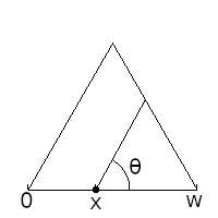
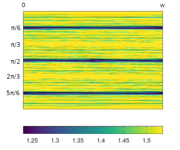
Figure 1: Image plot of equilateral triangle phase space under sequence length $m$=40, angular sequence function; note the y axis has been flipped, so that angle increases in the downward direction.

Sequence functions

A simple and useful sequence function can be constructed by considering only a given sequence’s symbol proportions. Given orbit sequence $S$ over alphabet $\mathcal{A}$, $|\mathcal{A}|=k$, let $n(\alpha)$ be the number of occurrences of $\alpha \in \mathcal{A}$ in $S$. Define symbol count vector, $v$ as: $v = [n(\alpha_1),…n(\alpha_k)]$. Let $u$ be the unit diagonal vector in $\mathbb{R}^k$: $u = [1/\sqrt(k),…,1/\sqrt(k)]$. Define the angular proportion measure as,

\(M_{\theta}(S) = \arccos((v/||v||)\cdot u).\)

The plot of Figure 1 used the sequence function $M_{\theta}$ on sequences of length $m=40$ at a resolution of $1000$ pixels on both dimensions. Note the angular measure’s output was ‘complemented’ by shifting $z:\rightarrow \pi/2-z$ so that sequences with more uniform symbol proportions had a higher score. This complementation for $M_{\theta}$ is used throughout the post. Note also in the plot the y axis has been flipped, which will be true for all phase space plots in this post. The colormap used for all plots is viridis.

Though the angular function is appealing for its simplicity, it only considers symbol proportions without regard to symbol ordering. Since one of the defining features of billiard orbits is their classification into periodic / non-periodic, a sequence function has some ability to detect periodicity would be useful. Here, we’ll use Lempel-Ziv compression, specifically LZ77. The LZ77 algorithm can employ a look-back window of arbitrary size, allowing very high compression for periodic symbolic sequences. For example, the periodic sequence $ABCABC…ABC$ at length $3n$ compresses to coded subsequence triples, $(0,1,’A’),(0,1,’B’),(0,1,’C’),(3,3(n-1),’A’)$ under LZ77. Call this sequence function $M_{LZ}$. As with $M_{\theta}$, complementation of this function with $z:\rightarrow c-z$ is used throughout the post, where $z$ is the compression level (in bytes). Such complementation highlights areas of high compression in the color plots.

As a third alternative, a regularity-based sequence function has been constructed by the author. The measure employs matrix products, and achieves a regularity score by comparing a test sequence to a set of repeating base patterns. This approach can be useful for picking out specific periodic patterns and their ‘neighbors’ in the bounce sequence phase space.

The regularity-based measure determines a distance between the sequence under test and concatenations of the base patterns by padding and splicing symbols of the test sequence under some penalty. The sequence under test undergoes some finite number of operations to match it to the base sequence(s), repeated over all possible padding and splicing operations (beyond just the Levenshtein distance). For instance, for a binary sequence we may have equiprobable templates $01$ and $10$. We compare test sequence $11110010101$ and all its subsequences to chains of the templates, ${010101…,101010…}$. Intuitively, the fewer bits we have to pad or splice in $11110010101$ to get to $0101…$ or $1010…$, the larger the score. The value assigned to the sequence is roughly monotone in a modified Levenshtein distance–one which charges a unit of penalty for splicing a symbol from the sequence, or padding a symbol into the sequence. Call this sequence function $M_{m}$.

The matrices of $M_m$ used in the plots correspond to a three-symbol equiprobable sequence, with parameter $\delta=0.1$:
\(S_a = \left[\begin{matrix} m_{a1} & 0 \\ 0 & m_{a2} \end{matrix}\right]; \hspace{0.7cm} S_b = \left[\begin{matrix} m_{b1} & 0 \\ 0 & m_{b2} \end{matrix}\right]; \hspace{0.7cm} S_c = \left[\begin{matrix} m_{c1} & 0 \\ 0 & m_{c2} \end{matrix}\right]\)
where,
\(m_{a1} = m_{a2} = \left[\begin{smallmatrix}3.433460498536983e-02&3.003814956109485e-02&9.011444868328456e-01\\ 1.111152264898700e-03&3.333456794696100e-02&3.703840882995666e-05\\ 3.703840882995666e-05&1.111152264898700e-03&3.333456794696100e-02\end{smallmatrix}\right]\)
\(m_{b1} = \left[\begin{smallmatrix}3.333456794696100e-02&3.703840882995666e-05&1.111152264898700e-03\\ 1.111152264898700e-03&3.333456794696100e-02&3.703840882995666e-05\\ 3.003814956109485e-02&9.011444868328456e-01&3.433460498536983e-02\end{smallmatrix}\right]\)
\(m_{b2} = \left[\begin{smallmatrix}3.333456794696100e-02&3.703840882995666e-05&1.111152264898700e-03\\ 9.011444868328456e-01&3.433460498536983e-02&3.003814956109485e-02\\ 3.703840882995666e-05&1.111152264898700e-03&3.333456794696100e-02\end{smallmatrix}\right]\)
\(m_{c1} = m_{b2}\)
\(m_{c2} = m_{b1}\)
(A technical note in reference to the original paper, the leftmost padding matrix $P$ is not included in the matrix products presented here; the $S_{\alpha}$ matrices here amount to $M_i P$ matrices in the paper’s notation. Nor do we normalize the matrix products to true probabilities.)

To compute the measure for, say, sample sequence $ABC$, the log of the norm of the corresponding matrix product is taken,

\(M_m(ABC) = \log||S_a S_b S_c||.\)

Each of these three measures has features that individually highlight different characteristics of the bounce sequences. They may also be combined, to yield more detailed information on the bounce sequences.

Further equilateral triangle plots

Consider again the bounce sequence over the whole phase space for an equilateral triangle. Figure 1 showed the image plot under sequence function $M_{\theta}$. Note again the angular measure’s output was “flipped,” by translating $z:\rightarrow \pi/2-z$. The resulting score range for the angular function is then approximately $[0.61548,\pi/2]$, where the lower bound is $\pi/2$ minus the maximal cone angle between the positive octant’s trace planes and the central diagonal.

Figure 2 shows an image plot of the same phase space for equilateral triangle orbits with sequences of length $40$ under the matrix product function $M_m$.

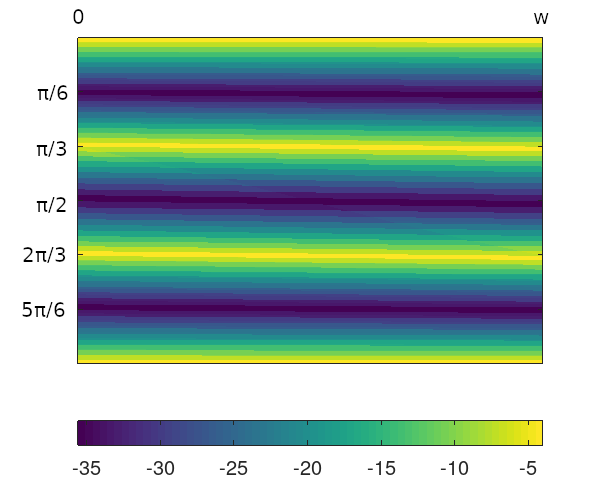
Figure 2: Image plot of equilateral triangle phase space under sequence length $m$=40, matrix regularity function $M_m$.

Compare with Figure 1. The matrix measure is highly banded, while the angular measure looks more disordered, and is largely at the equal-proportion end of the colormap (yellow). The differences are even more pronounced when examining a closeup. Figures 3 and 4 show respectively the angular and matrix functions under an equilateral triangle with sequences of length $40$ over the vertically narrowed region $[\pi/3,1.8]$x$(0,w)$.

Figure 3: Vertical zoom of phase space, to $[\pi/3,1.8]$x$(0,w)$ for the equilateral triangle under sequence length $m$=40, angular function.

Figure 4: Vertical zoom of phase space, to $[\pi/3,1.8]$x$(0,w)$ for the equilateral triangle under sequence length $m$=40, matrix function.

The angular measure in Figure 3 shows a solid band of yellow around $\pi/3$, with noticeable negatively sloped arcs cutting across the plot, with a particular focal point in the middle of the $\pi/2$ region. The matrix measure of Figure 4 still shows almost uniformly banded regions, with a slight downward slope. If you look closely, Figure 4 also has an arc, but it is much less pronounced than those under the angular measure.

The cause of the arcs may already be obvious to mathematical billiards people, while the banding may require a little more thought. The next sections will explain both these effects.

Billiard unfoldings

We’ll show that the arcs amount to initial conditions in the phase space that determine which side of a specific vertex the trajectory eventually hits, after some number of collisions. To better understand the arcs, it’s helpful to consider a typical method for easily visualizing orbits in a polygonal billiard.

Since the path of a billiard bouncing around inside a polygon can grow quite tangled, a typical scheme to aid in visualization is to leave the orbit trajectory a straight line and unfold the polygon around it. As many duplicate polygons are used as necessary, tiling a path that completely contains the straight trajectory [7]. If the polygon has rational angles, after tiling sufficiently many trajectories there is the added benefit of eventually exhausting every possible orientation of the original polygon with respect to rotations and reflections. The resulting finite set of rotated and reflected polygons can then be stitched together to create a compact manifold, which will contain all of the dynamics of the original table. This manifold is termed a translation surface. Billiard trajectories on the translation surface correspond to geodesic flows. On the other hand, if the polygon does not have rational angles, the manifold is not compact.

The equilateral triangle is a particularly simple example, it being one of the relatively few shapes that can tesselate the plane. See Figure 5 for a partial tesselation.

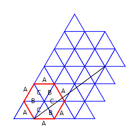
Figure 5: A partial tesselation of the plane with equilateral triangles. The hexagon highlighted in red amounts to a translation surface. The triangles composing the hexagon have their edges labelled consistently with the unfolding dynamic. The black line is a vertex-to-vertex path, termed a generalized diagonal. Translates of this line along the side amount to periodic orbits.

The associated translation surface, highlighted in red, is a hexagon. The sides of all triangles composing the hexagon have been labeled to match the unfoldings. Stitching together parallel sides (all labeled “A”) produces a flat torus. (After the first pair of sides is stitched, the intermediate cylinder is given a 180 degree twist; the remaining two pairs of sides can then be joined directly).

To better understand unfoldings and trajectories, consider Figure 6. Each trajectory has an angle $\theta$ equal to $1.3$ radians, while the foot point of the trajectory has been swept rightward in $(0,w)$.

The equilateral triangles actually form rhombic chains to cover the trajectories, similar to how squares in a lattice cover a line in $\mathbb{R}^2$ (as with Sturmian and Christoffel words). The rhombic segments follow the line by alternating between rhombuses oriented in the $\pi/3$ direction and in the $2\pi/3$ direction. As the foot point of the trajectory is shifted in the $x$ direction, the $\pi/3$, $2\pi/3$ changeover points gradually shift to contain the line.

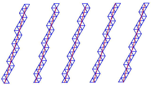
Figure 6: A series of trajectories depicted as unfoldings. All trajectories have angle $\theta=1.3$, while the foot point along the base side is swept from $0$ to $w$. The rhombic direction shifts move progressively to retain the trajectory in the unfolding as the foot point is varied.

In Figure 7 are some unfoldings with the foot point fixed at $0.5+\epsilon$, while the angle of the trajectory is varied between $\approx \pi/3$ and $\pi/2$. This has the unsurprising effect of increasing the number of $\pi/3$, $2\pi/3$ changeover points as $\pi/2$ is approached.

Figure 7: A series of trajectories depicted as unfoldings. All trajectories have constant foot point $x=0.501$ while the angle varies in $(\pi/3,\pi/2]$. More rhombic direction shifts are required as the angle approaches $\pi/2$.

With a bit more work, we can quantify the bounce sequences. Label each triangle’s sides and consider the simplest, ‘straight’ unfolding along the direction of $\pi/3$ in Figure 8. The bounce sequence can be read directly off the labeled sides, amounting to $ABCABC…$ and its left-shifts. As the angle is increased above $\pi/3$ we introduce rhombic direction shifts in the $2\pi/3$ direction. Labeling the sides again, we find each such shift merely interposes (or pads) another symbol ($A$, $B$, or $C$, depending on where the shift occurred) into the $ABCABC…$ sequence. The case is similar in all other directions, where the sequences may include $ACBACB…$ and its left-shifts as well.

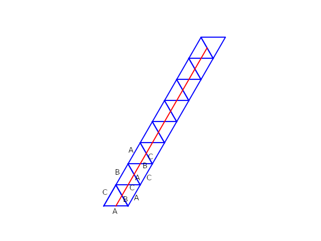
Figure 8: An unfolding along $\pi/3$, with initial triangles' sides labeled according to the unfoldings.

This padding effect as a function of trajectory angle now explains the banding effect in the $M_m$ sequence function of Figure 2 and Figure 4. If $M_m$ assigns a penalty to a sequence roughly proportional to the number of splices or pads required to make the sequence fully regular (to $ABCABC…$ or $ACBACB…$, and left-shifts), then the penalty would be proportional to the trajectory angle, mod the range $[0,\pi/6)$. The matrix function on the bounce sequence then acts to highlight the triangle’s angular information. The foot point information of the trajectory is almost completely lost.

The image plots in general are a result of the combination of the phase space sequences, and the nature of the sequence mapping. As we’ve just seen, the sequence function can have a major effect. We might even ask if for a given rational billiard, can we find a sequence function that similarly highlights aspects of the billiard boundary (to, say, always give us the interior angles), or flattens trajectory information (to, say, remove foot point position)?

In any case, for the remaining image plots in this post, the visual differences between the three sequence functions are less pronounced.

Branches of discontinuity

But what about the arcs, much more noticeable in Figure 3?

Consider again the $\pi/3$ “tunnel” of Figure 8. It is clear that all trajectories that pass through this tunnel of 16 triangles without touching the “sides” will have the same symbolic sequence prefix. A trajectory at exactly the angle $\pi/3$ will remain in the tunnel for all foot points in $(0,w)$. Also, any trajectory with angle $\pi/3 \pm \epsilon$ with $\epsilon$ sufficiently small, and the foot point placed appropriately in $(0,w)$, will fit. The total bundle of trajectories that fit into the tunnel correspond to a contiguous region in the $(x,\theta)$ phase space. If the sequence length is truncated to 16 in this case, that region under a colormap and any sequence measure will have a uniform color.

This tunnel effect also helps explain the width of the bands under the matrix $M_m$ mapping, and to a lesser extent the $M_{\theta}$ mapping.

At shorter sequence lengths, the tunnel, especially around $k\pi/3$, $k=0,1,2,…$, is physically wider. A wider tunnel corresponds to a larger bundle of trajectories that produce a given sequence, which produces a wider band in the image plot. The large yellow bands of both Figure 1 and Figure 2 result from the trajectories through the $\pi/3$ and $2\pi/3$ tunnels in the phase space, which produce perfectly proportioned, and perfectly regular bounce sequences.

The downward slope of the bands, especially evident in Figure 4, is a result of considering the tunnel limits as the foot point is swept rightward. The lower angle limit corresponds to a trajectory between the foot point and the rightmost vertex at the tunnel outlet (at top). As the foot point moves rightward, the angle of this limiting trajectory increases, which produces a downward sloping line on the $(x,\theta)$ plot. The upper angle limit is analagous, with the trajectory aimed at the leftmost vertex at the tunnel outlet.

Katok in [8] defines the boundaries of equal-prefix regions as branches of discontinuity. The sequence prefix partition of the phase space at some fixed sequence length is completely determined by the vertices encountered along any given trajectory’s unfolding.

Katok modifies the phase space slightly, employing ${\tau,x}$ coordinates where for trajectory angle $\theta$, $\tau = \cot(\theta)$. The importance of the cotangent will be seen shortly. The phase space under ${\tau,x}$ amounts to an infinite vertical strip: $(-\infty,\infty)$x$[0,w)$.

Figure 9 shows the plotting process for a single branch of discontinuity generated by a vertex visible from the base segment after two unfoldings. Shown in the left of the figure is the unfolding, with the vertex $v$ labeled. For each point $x$ on the base segment, we check if a line may be drawn through the existing unfoldings to reach the vertex.

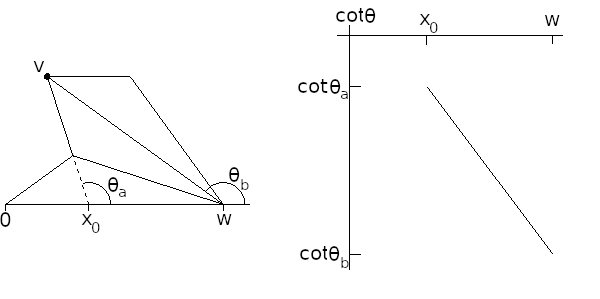
Figure 9: The set of trajectories that intersect vertex $v$ after 2 unfoldings may be depicted as a line segment in the cotangent phase space. Note that both endpoints' cotangents are negative.

Trajectories with foot points in the interval $(x_0,w)$ may be divided into two groups, depending on which side of the boundary line they fall on. (We discard the trajectory aimed directly at the vertex, which amounts to the discontinuity in question.) Each group will lead to a different unfolding, and correspondingly to a different bounce sequence.

It is evident that the cotangent of the angle between $v$ and $x$ changes linearly in $x$. This has the convenience of rendering branches of discontinuity as line segments in the cotangent phase space. Shown on the right side of the figure is the resulting branch. The region below the segment corresponds to trajectories that pass the vertex on the left, and the region above the segment corresponds to trajectories that pass the vertex on the right.

In general, to determine the branches of discontinuity up to some sequence length $m$, the unfoldings are performed one level at a time, beginning with the initial triangle. The initial triangle is then unfolded along the two sides opposite the base side. Each of the resulting two triangles are then unfolded along their two outward-facing sides, and so on. For each unfolded triangle, its outward vertex will describe a segment in the cotangent phase space if that vertex is visible from any point on the base triangle’s base side. (It is always possible that an unfolding places the new vertex out of sight along the unfolding path from the base side.)

In the limit in $m$, the closures of the regions contained within a given set of boundaries approach either single points, or horizontal line segments [8]. Since horizontal lines in the cotangent space map to horizontal lines in the angle space, the limiting regions are the same orientation in either case. For details see Katok [8].

Shown in Figure 10 and Figure 11 are branches of discontinuity associated with multiple vertex points positioned along two different lines. The regular spacing of the vertices in the unfolding translates to boundary segments focused around radiant points in the phase space. On the right side of Figure 10 are the branches of discontinuity as line segments in the cotangent phase space. Figure 11 shows the branches of discontinuity as arcs in the plain angular phase space. Note in this last plot the y axis has been reversed. Values increase in the downward direction, to match the orientation for the angular y axis in the color plots.

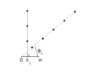
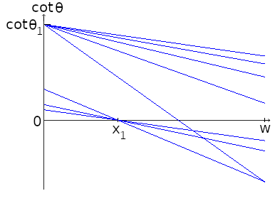
Figure 10: Discontinuity boundaries in the cotangent phase space corresponding to multiple colinear vertices in a (abstract) triangle unfolding.

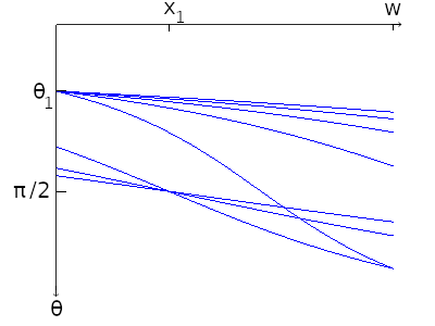
Figure 11: The angular phase space corresponding to the cotangent phase space in the previous figure. Note the y axis has been flipped, to match the orientation in the image plots.

Compare these focused ray plots with Figure 12, which shows a further closeup of Figure 3 around the $\pi/2$ region under the angular sequence function $M_{\theta}$:

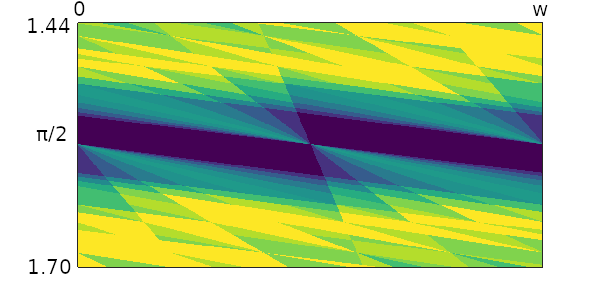
Figure 12: A closeup of the region around $\pi/2$ under angular sequence function on sequences of length $40$ for the equilateral triangle.

To better see the combined effect of the bounce sequences, boundaries of discontinuity, and the two sequence functions, let’s look at the orbits at angle $\theta \approx 1.55$ radians and foot points progressively farther to the left of $x=0.5$. These correspond to the ray regions of Figure 12 radiating upward and leftward from the central point at $(\pi/2,w/2)$.

x	orbit symbol sequence	symbol counts (A,B,C)
0.45	(C)BCABC(B)ABC(B)ABC(B)ABC(B)ABC(B)ABC(B)ABC(B)ABC(B)ABC(B)A	(10,19,11)
0.40	(C)BCA(C)BCA(C)BCABC(B)ABC(B)ABC(B)ABC(B)ABC(B)ABC(B)ABC(B)A	(10,17,13)
0.35	(C)BCA(C)BCA(C)BCA(C)BCABC(B)ABC(B)ABC(B)ABC(B)ABC(B)ABC(B)A	(10,16,14)
0.30	(C)BCA(C)BCA(C)BCA(C)BCA(C)BCA(C)BCABC(B)ABC(B)ABC(B)ABC(B)A	(10,14,16)
0.25	(C)BCA(C)BCA(C)BCA(C)BCA(C)BCA(C)BCA(C)BCABC(B)ABC(B)ABC(B)A	(10,13,17)

The sequences listed in the table have parentheses added to indicate “padding” symbols that break the otherwise regular $ABC…$ pattern. While the number of padding symbols in each sequence is the same, rendering the sequence’s values under the matrix sequence function $M_m$ nearly identical, the symbol proportions vary to some degree. This variation is picked up by the angular sequence function, coloring each ray region a different shade. The ray boundaries themselves are the discontinuity boundaries formed by the primary equilateral triangle vertex, located directly above the base side, and an infinitude of vertices directly above it, corresponding to successive upward unfoldings.

General results on rational billiards

At this point, it may be helpful to discuss some well-established results for billiards in rational polygons. Prominent results, for example, exist on the density of periodic and non-periodic orbits, and forms of ergodicity.

First, some definitions. Consider the general translation surface for a rational polygon. Define a generalized diagonal as a line segment connecting any two segments on the translation surface (Figure 5 depicted a short generalized diagonal under equilateral tesselation). For a point $p$ on a translation surface, let the (time) flow $\phi_t(p)$ be defined as the point arrived at after time $t$ along trajectory of some angle $\theta$. Let $\Upsilon$ be the interior of a rational polygon. Let $S^1$ be the 1-sphere.

The following results apply for rational polygons.

If we define the billiard phase space as $V = \Upsilon$x$S^1$, periodic points of the billiard flow are dense in $V$ [9].

If $G$ is the set of generalized diagonals then for any flow in a direction $\notin G$, the flow over the associated translation surface is dense [9].

As the generalized diagonals grow in length, their angles become approximately equidistributed in $S^1$ [10].

One may consider the interior-filling nature of the periodic orbits. Let $R$ be an arbitrary convex set within billiard surface $\Upsilon$. Define an $\epsilon$-well distributed periodic point as one whose orbit visits $R$ about as often in a given period as the ratio of the Lebesgue measure of $A$ to that of $\Upsilon$. The “about as often” is taken as an $\epsilon$ bound.

The set of $\epsilon$-well distributed periodic points is dense in phase space $V$ [9]. I.e. there are a lot of periodic points (foot point and angle) whose orbits fill the phase space at $\epsilon$ density. On the other hand, the set of directions whose orbits are not $\epsilon$-well distributed is at most a countable closed set [9]. So the set of periodic orbit directions that have trouble filling the whole space is at most countable in $S^1$.

We obtain even stronger results on periodic orbits and orbit densities for a special group of translation surfaces called lattice surfaces, a.k.a. Veech surfaces. Classes of triangles that have associated lattice surfaces include those of angle types $((k-1)\pi/(2k),(k-1)\pi/(2k), \pi/k)$, $k\ge3$, and others (see [13] for a recent list).

Define a uniquely ergodic direction as one for which all infinite trajectories are uniformly distributed. Formally, for a rectangle placed at right angle intersections to two parallel flows, the flows visit the rectangle the same proportion of time.

The Veech dichotomy states that each direction in the billiard flow is either completely periodic or uniquely ergodic. All lattice surfaces satisfy the Veech dichotomy (see e.g. [11]). So all trajectories not in $G$ are not just dense, but uniquely regodic. And that all trajectories in $G$ must have periodic orbits is a stronger statement than membership in $G$ merely being necessary for periodicity [8].

The 1,2,7 triangle and beyond

Now we’ll look at the $(1,2,7)$ triangle: a triangle with angles $(\pi/10,\pi/5,7\pi/10)$. The translation surface is shown in Figure 13. All parallel outer edges may be paired, and stitched together, to give a surface of total genus 4 [1]. The translation surface is also a lattice surface [12],[13], and therefore obeys the Veech dichotomy.

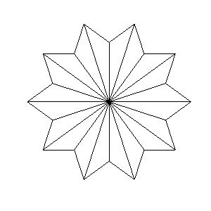
Figure 13: A fully unique unfolding of the $(1,2,7)$ triangle, around its smallest angle.

Figure 14 shows an image plot of the whole phase space under the LZ77 sequence function. (This and the remaining plots use sequence length $m=500$.) There are noticeable horizontal bands at increments of $\pi/10$. These angles coincide with the angles of the shortest generalized diagonals (consider Figure 13).

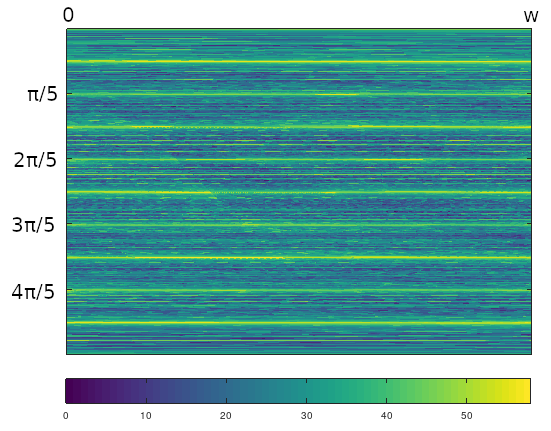
Figure 14: An image plot of the full phase space for the $(1,2,7)$ triangle, using LZ77 as the sequence function.

The angles of the set of generalized diagonals, $G$, indicate periodic orbits under the Veech dichotomy. Generalized diagonals are also the only directions that feature strictly colinear, regularly spaced vertices. Such colinear order gives rise to the focal ray structures we’ve seen in, for example, Figure 12. And the shortest generalized diagonals feature discontinuity boundaries with the largest vertical relief. Put another way, we saw from the section on branches of discontinuity that the longer the generalized diagonal, the more horizontal, and horizontally compressed, its discontinuity boundary segments, and hence its vertex ray structures become.

As a result, visually interesting structures will occur at angles equal to those of the generalized diagonals. And angles corresponding to longer generalized diagonals will require more magnification in the angular direction, to decompress the discontinuity boundary angles from nearly horizontal positions. Under appropriate vertical rescaling, since the angles of the generalized diagonals are dense in $S^1$, we expect every vertical span in the phase space to hold an infinite number of such focused ray figures.

In Figure 15 is a vertical closeup of the $9\pi/10$ generalized diagonal, using the matrix sequence function $M_m$. Recall that a periodic flow amounts to a trajectory angle for which all foot points are periodic (except the null set of trajectories that hit a vertex). The region just above and below $9\pi/10$ is fairly empty. Consider Figure 16, an unfolding along this angle. Notice that for every foot point along the bottom side of the base triangle, there are no vertices in the ‘hallway’ of this unfolding. So there are no boundaries of discontinuity as $x$ is varied at $9\pi/10$, and the structure in the image plot just around $9\pi/10$ is relatively plain.

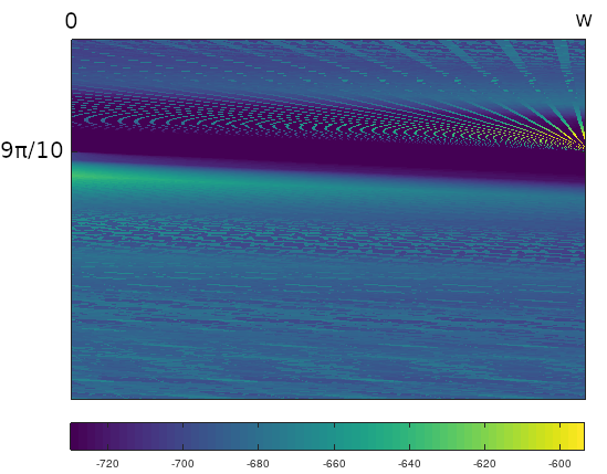
Figure 15: An image plot for the $(1,2,7)$ triangle, full width, with vertical zoom around the angle $9\pi/10,$ using matrix function $M_m$. Total height is $\approx \pi/50$.

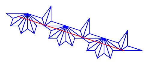
Figure 16: Unfolding the 1,2,7 triangle along the angle $9\pi/10$. The resulting "hallway," seen from the base side, has no interior singularities.

In contrast, consider Figure 17, which zooms in around the angle $7\pi/10$, also using $M_m$. Here, the “hallway” (not shown) features runs of vertices down its interior, and we obtain more interesting structures within the band around $7\pi/10$ on the image plot.

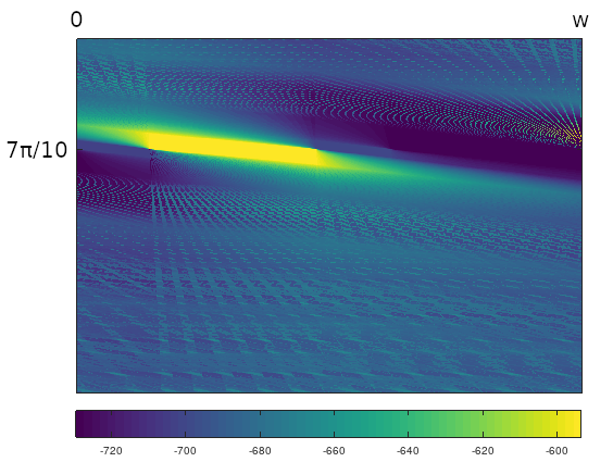
Figure 17: An image plot for the $(1,2,7)$ triangle, full width, with vertical zoom around the angle $7\pi/10,$ using matrix function $M_m$. Total height is $\approx \pi/50$.

In Figure 18, the same vertical zoom is retained, while some horizontal zoom is added. This corresponds to the left edge of the bright yellow band of Figure 17. The sequence function used is LZ77. The greater zoom shows some of the finer-scaled details. Note also some moiré effects in these zoomed-in images from aliasing in the rays.

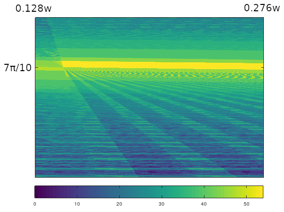
Figure 18: An image plot of the $(1,2,7)$ triangle, with horizontal zoom, and vertical zoom around $7\pi/10,$ using LZ77 compression for the sequence function.

A final comparison is worth mentioning before looking at other triangles. In Figure 19 is a plot of the same $7\pi/10$ closeup as Figure 18, but this time with a trio of $6$x$6$ matrices with entries randomly distributed in $[0.5,1.5]$. The resulting plot retains much of the detail of the LZ77 plot (as well as the same phase space region under $M_m$, which is not shown). Really, any sequence function that assigns sufficiently different values to different sequences will show distinct discontinuity domains in the phase space. However, the sequence function should also offer interpretable meaning to the values it assigns. For matrices with random entries, the meaning may be difficult to determine.

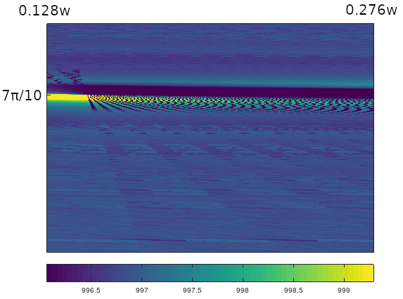
Figure 19: An image plot of the $(1,2,7)$ triangle, with horizontal zoom, and vertical zoom around $7\pi/10,$ using products of matrices with randomly-chosen entries for the sequence function. Compare with Figure 18.

The (1,2,20) triangle

To see how the dynamics vary further with triangle shape, the next four figures involve the $(1,2,20)$ triangle. This is still a Veech triangle, but it is more obtuse than the $(1,2,7)$ triangle. Figure 20 and Figure 21 show the total phase space plot for the $(1,2,20)$ triangle, under LZ77 compression and the matrix function $M_m$ respectively.

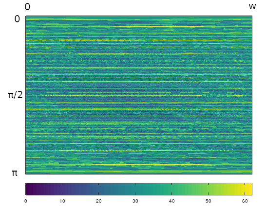
Figure 20: An image plot of the $(1,2,20)$ triangle over the whole phase space, under LZ compression sequence function.

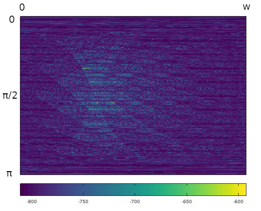
Figure 21: An image plot of the $(1,2,20)$ triangle over the whole phase space, using matrix sequence function $M_m$.

The plots in this case are more granular than for either the equilateral triangle or the $(1,2,7)$ triangle. Major bands occur at angular increments of $\pi/46$. Discontinuity boundary arcs and fine structure are more visible in the matrix sequence plot, in a pattern resembling fish scales. Modifying LZ77 sequence function output through a function that stretched out higher color values would likely help (not shown).

Figure 22 and Figure 23 show a vertical closeup for the $(1,2,20)$ triangle around the principal angle $19\pi/46$.

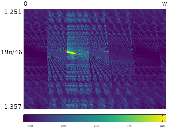
Figure 22: An image plot of the $(1,2,20)$ triangle under vertical zoom around the principal angle $19\pi/46$, using matrix sequence function $M_m$.

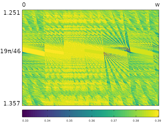
Figure 23: An image plot of the $(1,2,20)$ triangle under vertical zoom around the principal angle $19\pi/46$, using angular sequence function $M_{\theta}$.

Though the zoom level is about the same as in Figure 15 and Figure 17, there is more fine structure visible, with diffraction-like effects. This is consistent with the smaller smallest angle, $\pi/23$, and what this implies for tighter bunching of colinear vertices that give rise to the focal ray phenomenon.

Comparing Figure 22 and Figure 23, the angular function produces less distinct patterns in some areas than the matrix function, which is somewhat opposite the effects we saw in the equilateral triangle case. While the matrix measure reduced the equilateral phase plots to simple, horizontally banded regions, here the matrix measure is showing more contrast in fine-scale structure. The angular measure is purely projective of sequence ordering (i.e. it ignores it), while the matrix function accounts to some degree for both symbol proportion and ordering.

A last example

As a final example, recall that we expect that zooming in in the vertical (angular) direction should always reveal focal ray structures corresponding to increasingly longer generalized diagonals. We note the sequence length will correspondingly have to increase, since longer sequences are required to ‘reach,’ via unfoldings, vertices more distant from the base side.

In Figure 24 is a greater vertical zoom on a generalized diagonal at $\theta \approx 0.169861$, showing focal ray structures under the LZ77 sequence function. The height of the plot is about $\pi/500$ ($1/500$th the total height in Figure 14). The sequence length was kept at $500$, which at this scaling creates a somewhat blocky effect to the ray shapes. The image is also in vector graphics format (svg), which has the advantage over previous raster images of rendering cleaner lines.

Figure 24: An image plot for the $(1,2,7)$ triangle under high vertical zoom around the direction of a longer generalized diagonal, sequence length $500$, using LZ77 sequence function.

And the image plot at the top of this post? That image was made with a $(3,4,5)$ triangle, the plot centered around principal angle $7\pi/12$, with sequence function $M_m$.

All of the code for this project is available at the author’s GitHub repos: here and here.

References

[1]: H. Masur and S. Tabachnikov, Rational billiards and flat structures, in Handbook of Dynamical Systems, Elsevier, 1 (2002), 1015–1089.

[2]: Moon Duchin, Viveka Erlandsson, Christopher J. Leininger, Chandrika Sadanand, You can hear the shape of a billiard table: Symbolic dynamics and rigidity for flat surfaces. Comment. Math. Helv. 96 (2021), no. 3, pp. 421–463.

[3]: Aaron Calderon, Solly Coles, Diana Davis, Justin Lanier, Andre Oliveira, How to hear the shape of a billiard table, (preprint); retrieved July 2022 from the arXiv database, https://arxiv.org/abs/1806.09644.

[4]: J. Bobok and S. Troubetzkoy, Does a billiard orbit determine its (polygonal) table?, Fundamenta Mathematicae, 212 (2011), 129–144.

[5]: J. Bobok and S. Troubetzkoy, Code and order in polygonal billiards, Topology and its Applications, 159 (2012), 236–247.

[6]: Yang Shen, Jiazhong Yang, Hearing the shape of right triangle billiard tables, Discrete and Continuous Dynamical Systems, 2021, 41 (12) : 5537-5549.

[7]: Alex Wright, Bull. Amer. Math. Soc., 53 (2016), 41-56; published electronically: September 8, 2015.

[8]: A. Katok, The Growth Rate for the Number of Singular and Periodic Orbits for a Polygonal Billiard, Comm. Math. Phys. 111(1): 151-160 (1987).

[9]: Boshernitzan, Michael & Galperin, G. & Krüger, Tyll & Troubetzkoy, S.. (1998). Periodic billiard orbits are dense in rational polygons. Transactions of the American Mathematical Society. 350.

[10]: Benjamin Dozier. Equidistribution of saddle connections on translation surfaces. Journal of Modern Dynamics, 2019, 14: 87-120.

[11]: Smillie, John & Weiss, Barak. (2008). Veech’s dichotomy and the lattice property. Ergodic Theory and Dynamical Systems. 28. 1959 - 1972.

[12]: Clayton C. Ward, Calculation of Fuchsian groups associated to billiards in a rational triangle, Ergodic Theory Dynam. Systems 18 (1998), no. 4, 1019–1042.

[13]: Hooper, W. P. (2013). Another Veech Triangle. Proceedings of the American Mathematical Society, 141(3), 857–865.